Measures of dispersion

In this tutorial, we will explore the key measures of dispersion used in descriptive statistics: range, variance, and standard deviation. These measures help describe the spread or variability of data in a dataset.

By the end of this tutorial, you will understand what each measure of dispersion represents, how to calculate them, and when to use them. We will also provide practice questions to help reinforce your understanding.

1. Introduction to Measures of Dispersion

Measures of dispersion describe how spread out or scattered the values in a dataset are. While measures of central tendency (mean, median, mode) summarize the center of the data, measures of dispersion provide insights into the variability of the data. This is important because two datasets can have the same mean but different levels of variability, which can impact data interpretation.

The most common measures of dispersion are range, variance, and standard deviation.

2. What is the Range?

The range is the simplest measure of dispersion. It represents the difference between the highest and lowest values in a dataset, showing the total spread of the data.

2.1 Definition of Range

The range is the difference between the maximum and minimum values in a dataset. It provides a basic measure of the overall spread of the data, but it does not consider the distribution of the values between the extremes.

2.2 How to Calculate the Range

The formula for calculating the range is:

$\text{Range} = \text{Maximum Value} – \text{Minimum Value}$

For example, if the highest value in a dataset is 90 and the lowest value is 50, the range is:

$\text{Range} = 90 – 50 = 40$

2.3 When to Use the Range

The range is useful when you want a quick, general sense of the spread of data. However, it is sensitive to outliers, as a single extreme value can significantly affect the range. Therefore, it is not always the most reliable measure of dispersion for datasets with outliers.

3. What is the Variance?

Variance is a measure of dispersion that calculates how much each value in a dataset differs from the mean. Variance gives more weight to larger deviations from the mean, making it a good measure of variability, especially in datasets with widely spread values.

3.1 Definition of Variance

Variance is the average of the squared differences between each data point and the mean of the dataset. It provides insight into the overall variability of the data, but because the differences are squared, variance is not in the same unit as the original data (e.g., if the data are in units of dollars, the variance is in dollars squared).

3.2 How to Calculate the Variance

The formula for variance differs slightly depending on whether you are calculating it for a population or a sample.

Population variance: $\sigma^2 = \frac{\sum (x – \mu)^2}{N}$
Sample variance: $s^2 = \frac{\sum (x – \overline{x})^2}{n – 1}$

Where:

Σ(x – μ)²: The sum of the squared differences between each value and the population mean (μ).
Σ(x – x̄)²: The sum of the squared differences between each value and the sample mean (x̄).
N: The number of values in the population.
n – 1: The number of values in the sample minus 1 (this is known as Bessel’s correction and is used to provide an unbiased estimate of the population variance).

3.3 When to Use the Variance

Variance is useful when you want to understand the overall variability of a dataset, especially in datasets with large differences from the mean. However, because variance is in squared units, it is often less interpretable than standard deviation, which presents the variability in the same units as the original data.

4. What is the Standard Deviation?

The standard deviation is the square root of the variance. It provides a measure of dispersion in the same units as the original data, making it easier to interpret than variance. Standard deviation is widely used in public health and biostatistics to measure the variability or spread of data.

4.1 Definition of Standard Deviation

Standard deviation measures the average amount by which each data point differs from the mean. It is widely used because it is in the same units as the original data, making it easier to understand. A low standard deviation indicates that the data points are close to the mean, while a high standard deviation indicates that the data points are spread out over a wider range of values.

4.2 How to Calculate the Standard Deviation

The formula for standard deviation is:

Population standard deviation: $\sigma = \sqrt{\frac{\sum (x – \mu)^2}{N}}$
Sample standard deviation: $s = \sqrt{\frac{\sum (x – \overline{x})^2}{n – 1}}$

Where:

Σ(x – μ)²: The sum of the squared differences between each value and the population mean (μ).
Σ(x – x̄)²: The sum of the squared differences between each value and the sample mean (x̄).
N: The number of values in the population.
n – 1: The number of values in the sample minus 1.

4.3 When to Use the Standard Deviation

Standard deviation is used when you need a measure of variability that is easy to interpret. It is useful for comparing the spread of data between different datasets and for understanding the typical amount by which data points deviate from the mean.

5. Practice Questions

Test your understanding of the measures of dispersion with these practice questions. Try answering them before checking the solutions.

Question 1:

A dataset contains the following values: 10, 15, 20, 25, 30. What is the range?

Answer 1:

Answer, click to reveal

$\text{Range} = 30 – 10 = 20$

Question 2:

A dataset contains the values 5, 7, 8, 10, and 12. Calculate the variance (sample variance).

Answer 2:

Answer, click to reveal

Step 1: Find the mean: $\overline{x} = \frac{5 + 7 + 8 + 10 + 12}{5} = 8.4$

Step 2: Subtract the mean from each value and square the result: $(5 – 8.4)^2 = 11.56$ , $(7 – 8.4)^2 = 1.96$ , $(8 – 8.4)^2 = 0.16$ , $(10 – 8.4)^2 = 2.56$ , $(12 – 8.4)^2 = 12.96$

Step 3: Sum the squared differences: $11.56 + 1.96 + 0.16 + 2.56 + 12.96 = 29.2$

Step 4: Divide by (n – 1): $s^2 = \frac{29.2}{4} = 7.3$

Question 3:

A sample has a variance of 9. What is the standard deviation?

Answer 3:

Answer, click to reveal

$s = \sqrt{9} = 3$

6. Conclusion

Measures of dispersion—range, variance, and standard deviation—are critical tools in descriptive statistics that help us understand the spread or variability of data. While the range provides a quick overview of the data spread, variance and standard deviation offer more detailed insights into how data points deviate from the mean.

Remember:

The range gives the difference between the maximum and minimum values but is sensitive to outliers.
The variance measures the average squared deviation from the mean, but its units are not the same as the original data.
The standard deviation is the square root of the variance and is in the same units as the original data, making it easier to interpret.

Final Tip for the CPH Exam:

Make sure you understand how to calculate and interpret each measure of dispersion, and how they are used in studies.

Humanities Moment

The featured image for this article is Öland (1912) by Helge Johansson (Swedish, 1886–1926). Unfortunately, despite Johansson’s artwork showing up at multiple auctions and the works garnering thousands of dollars, there is very little biographical information available.

Mean, median and mode

In this tutorial, we will explore the three primary measures of central tendency: the mean, median, and mode. These statistical tools are used to summarize data by identifying a central point or typical value in a dataset.

By the end of this tutorial, you will understand what each measure of central tendency represents, how they are calculated, and when to use them. We will also provide practice questions to help reinforce your understanding.

1. Introduction to Descriptive Statistics

Descriptive statistics provide a way to summarize and describe the main features of a dataset. Measures of central tendency—mean, median, and mode—are used to identify a single value (or in many cases, a set of values) that represents the center of the data. These measures give us insight into where the majority of data points lie and help us understand the overall pattern in the dataset.

Each measure of central tendency has its own strengths and weaknesses, and it is important to choose the right one depending on the data distribution and the context of the analysis.

2. What is the Mean?

The mean (often referred to as the average) is the most commonly used measure of central tendency. It represents the arithmetic average of a set of values and is calculated by summing all the values in the dataset and then dividing by the number of values.

2.1 How to Calculate the Mean

The formula for calculating the mean is:

$\text{Mean} = \frac{\sum{x}}{n}$

Where:

Σx: The sum of all values in the dataset.
n: The number of values in the dataset.

2.2 When to Use the Mean

The mean is useful when you have a dataset without extreme outliers and when you want to take all values into account. It provides a comprehensive measure of central tendency but can be misleading if the data are heavily skewed by outliers.

3. What is the Median?

The median is the middle value in a dataset when the values are arranged in ascending or descending order. If the dataset has an odd number of values, the median is the middle value; if the dataset has an even number of values, the median is the average of the two middle values.

3.1 Definition of the Median

The median is the value that separates the dataset into two equal halves: 50% of the data points are smaller than the median, and 50% are larger. The median is not affected by outliers, making it a better measure of central tendency for skewed distributions.

3.2 How to Calculate the Median

To calculate the median:

Step 1: Arrange the data in ascending order.
Step 2: If the number of values is odd, the median is the middle value.
Step 3: If the number of values is even, the median is the average of the two middle values.

3.3 When to Use the Median

The median is useful when the dataset contains outliers or when the data are skewed. It provides a more accurate representation of the center of the data in these situations compared to the mean.

4. What is the Mode?

The mode is the value that appears most frequently in a dataset. Unlike the mean and median, the mode can be used for both numerical and categorical data. A dataset may have more than one mode (bimodal or multimodal) if multiple values occur with the same highest frequency.

4.1 Definition of the Mode

The mode is the value that occurs most often in a dataset. In some cases, there may be no mode if no value repeats, or there may be multiple modes if several values have the same frequency.

4.2 How to Calculate the Mode

To calculate the mode:

Step 1: Identify the value(s) that occur most frequently in the dataset.
Step 2: The value(s) with the highest frequency is the mode.

4.3 When to Use the Mode

The mode is useful for categorical data (e.g., identifying the most common category) or for datasets with repeated values. It is less commonly used for continuous data unless you want to identify the most frequent value.

5. Practice Questions

Test your understanding of the measures of central tendency with these practice questions. Try answering them before checking the solutions.

Question 1:

A dataset contains the following values: 2, 4, 4, 5, 7, 8, 10. What is the mean of this dataset?

Answer 1:

Answer, click to reveal

$\text{Mean} = \frac{2 + 4 + 4 + 5 + 7 + 8 + 10}{7} = \frac{40}{7} \approx 5.71$

Question 2:

The following values represent the number of hours worked by a group of individuals: 20, 25, 30, 35, 40. What is the median?

Answer 2:

Answer, click to reveal

Since there is an odd number of values, the median is the middle value, which is 30.

Question 3:

A set of test scores contains the following values: 85, 90, 90, 95, 100. What is the mode?

Answer 3:

Answer, click to reveal

The mode is 90, as it appears more frequently than the other values.

6. Conclusion

Measures of central tendency—mean, median, and mode—are fundamental tools in descriptive statistics that help summarize data by identifying its central point. Each measure has its own strengths and is appropriate for different types of data or distributions. Choosing the right measure of central tendency depends on the characteristics of the data, such as whether the data include outliers or are skewed.

Remember:

The mean is best used for datasets without outliers, as it accounts for all data points.
The median is best for skewed datasets or those with outliers, as it is less affected by extreme values.
The mode is useful for categorical data or when identifying the most frequent value in a dataset.

Final Tip for the CPH Exam:

Ensure you understand how to calculate and interpret each measure of central tendency. In particular, keep in mind what might be the best for situations with normal distributions, skewed distributions, and so on.

Humanities Moment

The featured image for this article is Albicocca Alessandrina a Mandorla Amara. [Armeniaca Alexandrina ; Apricot (1817-1839) by Giorgio Gallesio (Italian, 1772-1839). Giorgio Gallesio, an 18th-19th century Italian botanist, specialized in citrus and authored the influential Traité du citrus, which challenged prevailing ideas by showing hybrids result from outcross pollination, not grafting. He also explored species compatibility and coined the term “dominant” in hereditary studies, cementing his legacy in botany and genetics.

Create Leaflet maps with Folium and GeoPandas

Introduction

Welcome to this PyFriday tutorial! Today, we're diving into a project where we'll use Python to create an interactive map that shows critical health infrastructure across the United States. Imagine you've been assigned a project to understand the distribution of two types of hospitals:

Level I Trauma Centers: These are hospitals with the highest capability to handle emergency trauma cases.
General Hospitals with 100+ Beds: These hospitals are large enough to handle significant patient loads.

Our goal is to help public health analysts quickly understand where these resources are located, providing insights into how well regions are served by medical facilities. In this tutorial, we will be using Folium for mapping,GeoPandas for handling geographic data, and Pandas for data processing. Let’s get started with a step-by-step approach!

1. Importing Necessary Libraries

The first step in any Python project is to import the necessary libraries. Here, we're using Folium, GeoPandas, and Pandas:

GitHub Gist

Each library has its unique role in this project:

folium: This helps create interactive maps that you can view in a web browser.
pandas: Used for handling and analyzing data, allowing us to manage non-geographic parts of our datasets.
geopandas: Extends Pandas to include spatial data, which is essential for working with maps and geographic information.

2. Loading the Data

Next, we load the hospital and county boundary data. This includes a GeoJSON file for hospitals and a shapefile for county boundaries:

GitHub Gist

hospitals = gpd.read_file(): This command reads a GeoJSON file containing hospital information.
counties = gpd.read_file(): This command reads a shapefile with county boundaries, which helps us identify the geographic regions we are mapping.

You may have noticed they're the same command; GeoPandas read_file() can take multiple file types due to the nature of the function itself. Both datasets are loaded into GeoDataFrames, which are like Pandas DataFrames but are specially designed to work with geographic data.

3. Handling JSON Serialization Issues

Sometimes, the hospital data contains columns that cannot be directly converted into JSON format, such as datetime fields. This can cause issues when adding data to the map, and unlucky for us, we have some datetime objects in our geojson data. To solve this, we convert any datetime columns to strings:

GitHub Gist

For the above chunk, we're using hospitals.select_dtypes(include=['datetime', 'datetimetz']) to go into the hospitals DataFrame, then selecting any columns with the data type of datetime or the alternative datetimetz, and once these are selected, we simply use the hospitals[column] = hospitals[column].astype(str) to reassign the type from a date type to a type of string. By converting datetime fields to strings, we make the data compatible for visualization. Folium uses GeoJSON, which requires all data to be serializable (i.e., easy to convert into a JSON format that the browser can read).

4. Filtering the Data for Specific Criteria

General Hospitals with 100+ Beds

We only want to display general medical and surgical hospitals with 100 or more beds, as these represent significant healthcare resources:

GitHub Gist

Here, we use filtered_hospitals_points to create a new dataset from the hospitals data, but only keep rows that match our conditions:

The hospital must be of type “GENERAL MEDICAL AND SURGICAL HOSPITALS”.
It must have at least 100 beds.

This ensures that our map only shows larger hospitals capable of handling more patients. As an aside, this also greatly reduces the amount of data being used, and thus the end product will be more manageable. To create an end product for all hospitals in a way similar to how we're doing it would create an interactive map over 10GB in size.

5. Adding Tooltips for Hospital Information

To make our map interactive, we add tooltips. A tooltip is the information box that pops up when you hover over a point on the map. We add details like hospital name, address, and bed count:

GitHub Gist

The tooltips give more context to users of the map. You'll notice that within the pop-up, html is used for bolding and creating new lines, and we can call values to be displayed by pointing to the column name, with the row being the location being clicked on.

6. Creating the Base Map

Now it’s time to create our base map. We will center it on the USA, with a zoom level of 5:

GitHub Gist

Explanation for New Users: The folium.Map() function creates a basic map that will serve as the canvas. We use:

location=[39.8283, -98.5795] to center the map roughly over the USA.
zoom_start=5 sets the initial zoom level, giving a wide view of the country. Feel free to mess around with this setting to find your preferred view.

7. Adding Hospital Data to the Map

We can now add a layer to display the general hospitals with 100+ beds. This layer will be initially hidden so users can choose to see it:

GitHub Gist

We use folium.FeatureGroup to create this group of features (in this case, hospital points).

8. Visualizing Trauma Level I Facilities by County

Now we’ll add information about Level I trauma facilities, focusing on county-level aggregation:

GitHub Gist

We filter the hospital data to only include hospitals with Level I trauma centers.
We then count how many such hospitals exist in each county using groupby and merge the results with our county data.
For any counties that have no Level I trauma centers, we then fill the NA values with 0.
This gives us the data we need to create a choropleth layer, showing which counties have Level I trauma facilities.

9. Adding Styling and Tooltips for Trauma Layers

To make the trauma data more visually informative, we define a color scale based on the number of Level I trauma centers in each county. This helps users quickly see which areas may have potential gaps or much higher expenses associated with accessing care.

GitHub Gist

We use different shades of color to visually communicate the distribution of trauma facilities. The darker the color, the more trauma centers are present in that county. We also are joining our hospital locations to our county layer, making it so that users can see exactly where facilities are, alongside a count of how many facilities are available by county.

10. Adding a Custom Legend

A map is much easier to interpret if it has a legend that explains the color coding. We add a custom HTML legend to the map:

GitHub Gist

This custom HTML legend helps users understand what the different colors on the map represent, making it much more intuitive to interpret. There is a weakness to this approach in that it won't adjust if there's a sudden influx or removal of facilities, but considering the fact most Trauma I facilities last for decades and take a long time to build, this isn't so much of a concern here.

11. Finalizing the Map with Layer Control and Saving

To complete our interactive map, we add a layer control widget that allows users to toggle between different layers:

GitHub Gist

Finally, we save the map to an HTML file so it can be viewed in a web browser:

GitHub Gist

Saving the map as an HTML file means that anyone with a browser can view it. It also makes sharing easy, allowing the map to be embedded in websites or shared directly. It should be noted though that depending on the size of your map, some ways of sending data (e.g. email) may not be ideal.

Checking Results

Now that we have a map, let's open it up and check our results. Keep in mind you can adjust layers using the sandwich marker on the right hand side.

Open the interactive map in a new tab. This historical tutorial output is approximately 37 MB and may take time to load. It is not a current directory of hospital services.

Conclusion and Further Improvements

Congratulations on completing this project! You now have a functional, interactive map that provides insights into the distribution of major hospitals and trauma centers in the United States. This project has covered some core concepts:

Loading and cleaning geospatial data
Using Folium and GeoPandas to create interactive maps
Adding informative layers and tooltips to enhance map usability

Ideas for Further Development

Add Real-Time Data: Integrate live data feeds (e.g., emergency response units) to make the map dynamic and responsive to ongoing events.
Additional Data Layers: Add new layers, such as healthcare shortages or hospital capacity updates, to provide a more comprehensive view.
Filter Options: Allow users to filter hospitals by bed count, type, or other criteria through an interactive interface.
Enhanced Styling: Experiment with different color scales or icons to improve visual aesthetics and clarity.

We hope this tutorial has helped you feel more comfortable with mapping in Python! Keep in mind this is an entire field on its own, so there's plenty more to learn!

References

Humanities Moment

The featured image for this article is Boy with Map of Scandinavia (1771) by Ulrika Pasch (Swedish, 1735-1796). Ulrika "Ulla" Fredrica Pasch was a prominent Swedish Rococo painter and miniaturist. Born into an artistic family, she was the daughter of painter Lorens Pasch the Elder and the sister of Lorens Pasch the Younger. Trained by her father, Ulrika began her professional career in the 1750s, eventually establishing her own studio and clientele. In 1773, she became the only female member inducted into the Royal Swedish Academy of Arts that year. Throughout her career, Pasch was commissioned by members of the Swedish aristocracy and royal court, earning recognition as one of the most successful female artists in Sweden before the 19th century.

Causal inference in public health

In this tutorial, we will explore the concept of causal inference in public health research. Causal inference refers to the process of determining whether an observed association between an exposure and an outcome reflects a true causal relationship. This process is essential in epidemiology because public health interventions rely on accurate identification of causal factors that impact health outcomes. Understanding causal inference is key for the Certified in Public Health (CPH) exam and for interpreting research that informs public health decisions.

By the end of this tutorial, you will understand the importance of causal inference, the methods used to establish causality, and the challenges involved in determining causality in public health research. Practice questions are included to reinforce your knowledge.

1. Introduction to Causal Inference

Causal inference refers to the process of determining whether an exposure causes an outcome. It involves evaluating whether changes in one variable (e.g., smoking) lead to changes in another variable (e.g., lung cancer). While observational studies often reveal associations between exposures and outcomes, they do not necessarily imply causality. Causal inference requires careful consideration of the evidence and the use of appropriate methods to rule out alternative explanations such as confounding, bias, or random chance.

2. Why is Causal Inference Important in Public Health?

In public health, understanding the cause of health outcomes is critical for designing effective interventions and policies. If we can identify a true cause of a health issue, we can take action to prevent it. However, if the cause is incorrectly identified due to improper causal inference, interventions may be ineffective or even harmful. For example, knowing that smoking causes lung cancer has led to significant public health campaigns and policies to reduce smoking rates, saving countless lives.

Accurate causal inference allows public health professionals to:

Implement effective interventions to reduce disease and improve health.
Allocate resources efficiently to address the true causes of health problems.
Avoid the implementation of ineffective or harmful interventions based on incorrect assumptions.

3. Challenges in Establishing Causality

Establishing causality in public health research can be difficult due to several challenges:

Confounding: A confounder is a variable that is associated with both the exposure and the outcome, which can distort the observed relationship. For example, age might confound the relationship between physical activity and heart disease if older individuals are less active and more prone to heart disease.
Bias: Bias can distort study results in various ways, including selection bias (when the sample is not representative) and information bias (when data are collected or measured inaccurately).
Reverse Causality: Sometimes, the outcome may influence the exposure, rather than the exposure influencing the outcome. For example, individuals with undiagnosed heart disease may reduce their physical activity due to fatigue, creating a false association between low physical activity and heart disease.
Ethical Constraints: In many cases, it is unethical to conduct experiments that would provide the most definitive evidence for causality. For instance, exposing people to harmful substances in a randomized controlled trial (RCT) would be unethical.

4. Methods for Causal Inference

Several methods are used to establish causal relationships in public health research. While no single method can definitively prove causality, the combination of evidence from multiple sources strengthens the case for a causal relationship.

4.1 Experimental Studies (Randomized Controlled Trials)

Randomized controlled trials (RCTs) are considered the gold standard for establishing causality. In RCTs, participants are randomly assigned to receive either an intervention or a control (e.g., placebo). Randomization helps to evenly distribute confounders across the groups, reducing the risk of bias and allowing researchers to draw stronger conclusions about the causal effect of the intervention on the outcome.

However, RCTs are often impractical or unethical in public health research, especially for harmful exposures like smoking or pollution.

4.2 Observational Studies (Cohort and Case-Control Studies)

Cohort studies and case-control studies are the most common types of observational studies used in public health research. While these studies cannot definitively establish causality, they provide valuable evidence about associations between exposures and outcomes.

Cohort Studies: Follow a group of individuals over time to assess whether exposure to a risk factor increases the likelihood of developing an outcome. They are useful for establishing temporality (i.e., the exposure precedes the outcome).
Case-Control Studies: Compare individuals with a disease (cases) to those without the disease (controls) to assess whether past exposure to a risk factor is associated with the disease. These studies are useful for studying rare diseases but are prone to recall bias.

4.3 Statistical Methods for Adjusting for Confounding

Confounding can distort the relationship between an exposure and an outcome, making it appear that there is a causal relationship when there is not. To address confounding, researchers use statistical methods to adjust for confounders and isolate the effect of the exposure.

Multivariable regression: Involves including potential confounders as covariates in the model to control for their effects.
Stratification: Analyzing the data within strata (e.g., age groups) to control for confounding and better understand the exposure-outcome relationship.
Propensity score matching: A method that matches individuals with similar characteristics to create groups that are comparable with respect to confounders.

4.4 Hill’s Criteria for Causation

Hill’s criteria for causation provide a framework for evaluating whether an observed association is likely to be causal. These nine criteria include:

Strength of association: A strong association is more likely to be causal than a weak one.
Temporality: The exposure must occur before the outcome for a causal relationship to exist.
Consistency: Repeated observations of the association in different studies and populations strengthen the case for causality.
Biological gradient: A dose-response relationship, where greater exposure leads to greater risk, supports causality.
Plausibility: The association should make biological sense based on current scientific knowledge.
Coherence: The association should align with what is already known about the disease.
Specificity: The exposure leads to a specific outcome, although this is not always necessary.
Experiment: Experimental evidence, such as from RCTs, can provide strong support for causality.
Analogy: If a similar exposure is known to cause the outcome, it supports the likelihood of a causal relationship.

5. Practice Questions

Test your understanding of causal inference with these practice questions. Try answering them before checking the solutions.

Question 1:

A study finds that individuals who exercise regularly have a lower risk of heart disease. However, individuals who exercise may also eat healthier diets and be wealthier. What issue does this example highlight?

Answer 1:

Answer, click to reveal

This example highlights the issue of confounding, where factors such as diet and wealth may influence the relationship between exercise and heart disease, potentially distorting the observed association.

Question 2:

A randomized controlled trial finds that a new medication reduces blood pressure in individuals compared to a placebo. What method was used to minimize confounding in this study?

Answer 2:

Answer, click to reveal

Randomization was used to minimize confounding by evenly distributing potential confounders across the treatment and placebo groups.

Question 3:

A researcher uses multivariable regression to adjust for age and smoking status when examining the relationship between alcohol consumption and liver disease. What is the researcher trying to control for?

Answer 3:

Answer, click to reveal

The researcher is trying to control for confounding by adjusting for age and smoking status, which could influence the relationship between alcohol consumption and liver disease.

6. Conclusion

Causal inference is a critical process in public health research, allowing researchers to determine whether observed associations are truly causal. While it is challenging to establish causality, the combination of evidence from randomized controlled trials, observational studies, and statistical methods can provide strong support for causal relationships.

Remember:

Randomized controlled trials provide the strongest evidence for causality by minimizing confounding and bias.
Observational studies are useful for identifying associations, but they require careful consideration of confounding and bias.
Statistical methods such as multivariable regression and stratification help control for confounding and provide more accurate estimates of causal effects.
Hill’s criteria for causation offer a framework for evaluating whether an observed association is likely to be causal.

Final Tip for the CPH Exam:

Make sure you understand the various methods used for causal inference and the challenges involved in establishing causality. Practice applying these methods to different research scenarios, as this knowledge is crucial for answering questions related to causality in the Certified in Public Health (CPH) exam.

Humanities Moment

The featured image for this CPH Focus is Anacardium occidentale (1909) by Ellen Isham Schutt (American, 1873 – 1955). Schutt was an American botanical illustrator renowned for her contributions to the U.S. Department of Agriculture’s Pomological Watercolor Collection, painting over 700 detailed watercolors of fruits and nuts. Born in Arlington, Virginia, she was also an early resident of Cherrydale, where she built a notable neoclassical home and contributed to genealogical research. Her precise illustrations, often highlighting fruit imperfections, supported agricultural studies and reflected Progressive Era ideals of nature control. Later, she painted an extensive series of apples for the University of California and modeled fruit in wax to study preservation. Schutt’s legacy endures through her detailed botanical art.

Association versus causation

In this tutorial, we will explore the critical distinction between association and causation in epidemiology. While association refers to a statistical relationship between two variables, causation means that one variable directly influences another. Understanding this difference is crucial for public health professionals, as it affects how research findings are interpreted and how public health policies are shaped. This topic is also essential for the Certified in Public Health (CPH) exam.

By the end of this tutorial, you will understand the concepts of association and causation, the challenges in establishing causality, and the importance of this distinction in public health research. Practice questions are provided to reinforce your knowledge.

1. Introduction to Association and Causation

In epidemiology, researchers often observe a relationship between two variables, such as an exposure (e.g., smoking) and an outcome (e.g., lung cancer). However, the presence of an association between these variables does not necessarily mean that one causes the other. Causation implies that changes in one variable directly result in changes in another. Distinguishing between association and causation is fundamental for making accurate public health recommendations and implementing effective interventions.

2. What is Association?

Association refers to a statistical relationship between two variables. If two variables are associated, it means that changes in one variable are related to changes in another. However, association does not imply that one variable causes the other; it merely indicates that they are linked in some way.

2.1 Definition of Association

An association between two variables exists when the occurrence or level of one variable is related to the occurrence or level of another variable. Associations can be positive (both variables increase or decrease together) or negative (as one variable increases, the other decreases).

Positive association: Increased physical activity is associated with lower rates of heart disease.
Negative association: Higher levels of education are associated with lower rates of smoking.

2.2 Examples of Association

Example 1: Studies show an association between high sugar intake and an increased risk of obesity. However, this does not prove that sugar intake directly causes obesity, as other factors like genetics or physical activity might also play a role.
Example 2: A study finds an association between watching television and aggressive behavior in children. This association could be due to other factors, such as parental involvement or socioeconomic status, rather than a direct causal link between television and aggression.

3. What is Causation?

Causation refers to a direct relationship between two variables, where changes in one variable directly result in changes in another. For example, if smoking causes lung cancer, this means that smoking directly increases the risk of developing lung cancer, regardless of other factors.

3.1 Definition of Causation

Causation occurs when there is sufficient evidence to show that changes in an exposure lead directly to changes in the outcome. Establishing causality requires more than just an observed association; it also involves demonstrating that the exposure precedes the outcome and that the relationship is not explained by other factors.

3.2 Challenges in Establishing Causation

While associations are relatively easy to identify in observational studies, establishing causation is much more difficult. The following are some key challenges in determining causality:

Confounding: Confounding occurs when an outside factor is related to both the exposure and the outcome, distorting the relationship between them. For example, age could confound the relationship between physical activity and heart disease, as older individuals may be less active and at higher risk of heart disease.
Temporality: For causality to be established, the exposure must occur before the outcome. If researchers cannot clearly establish the temporal sequence of events, it is difficult to determine whether the exposure caused the outcome.
Bias: Selection bias, information bias, and other forms of bias can distort study results, making it appear that there is a causal relationship when there is not.
Chance: Sometimes associations occur by chance, particularly in studies with small sample sizes. Random variation can lead to spurious associations that do not reflect a true causal relationship.

4. Methods to Assess Causality

To assess whether an association is likely to be causal, researchers use several methods, including:

Hill’s Criteria for Causation: These nine criteria (including strength of association, consistency, temporality, and biological plausibility) help evaluate whether an association is likely to be causal.
Experimental Studies: Randomized controlled trials (RCTs) provide the strongest evidence for causality, as participants are randomly assigned to exposure groups, allowing researchers to control for confounding factors.
Longitudinal Studies: Following participants over time in cohort studies allows researchers to establish temporality and reduce the risk of confounding, making it easier to infer causality.
Statistical Adjustment: Techniques such as multivariable regression can help control for confounding factors, allowing researchers to isolate the effect of the exposure on the outcome.

5. Practice Questions

Test your understanding of the difference between association and causation with these practice questions. Try answering them before checking the solutions.

Question 1:

A study finds that people who drink more coffee tend to have lower rates of depression. Can we conclude that drinking coffee prevents depression?

Answer 1:

Answer, click to reveal

No, this study demonstrates an association between coffee consumption and lower rates of depression, but it does not prove causation. Other factors, such as lifestyle or genetics, may be involved in the relationship.

Question 2:

A clinical trial randomly assigns participants to either receive a vaccine or a placebo. After two years, the vaccinated group has a significantly lower rate of infection compared to the placebo group. Can this study conclude causality?

Answer 2:

Answer, click to reveal

Yes, this randomized controlled trial provides strong evidence for causality, as participants were randomly assigned to exposure groups, reducing the risk of bias and confounding. The vaccine likely caused the reduction in infection rates.

Question 3:

A study finds that people who eat more vegetables have lower rates of heart disease. However, people who eat vegetables also tend to exercise more and have higher incomes. What issue might complicate the interpretation of this association?

Answer 3:

Answer, click to reveal

This is an example of confounding, where factors such as exercise and income may be influencing the relationship between vegetable consumption and heart disease. These factors need to be controlled for to assess whether the association is causal.

6. Conclusion

In epidemiology, it is essential to distinguish between association and causation. While associations are often observed in studies, they do not necessarily imply that one variable causes the other. Establishing causality requires a more rigorous evaluation, including demonstrating that the exposure precedes the outcome, ruling out confounding factors, and providing evidence from experimental or longitudinal studies.

Remember:

An association between two variables means they are statistically related, but this does not imply that one causes the other.
Causation requires evidence that the exposure directly leads to the outcome and that the relationship is not due to confounding, bias, or chance.
Methods such as Hill’s criteria for causation, randomized controlled trials, and longitudinal studies help determine whether an observed association is likely to be causal.

Final Tip for the CPH Exam:

Make sure you understand the distinction between association and causation. One helpful exercise is skimming science news articles, and then reading the underlying studies. Did the author of the article state causation from association? Or were they accurate to the source material? How do you know? This distinction is crucial for interpreting research findings and making sound public health decisions, and will be tested on the Certified in Public Health (CPH) exam.

Humanities Moment

The featured image for this CPH Focus is Histoire naturelle des champignons Pl.54 (1883) by Guillaume Sicard (French, 1829-1886). Sicard actually has very little known of himself aside from his work being published within Histoire naturelle des champignons, or “The Natural History of Mushrooms”. This is particularly interesting as the work itself has been seen as a critical work of plant and fungus taxonomical art.

Epi Explained: What are Epi Curves?

An Epidemic Curve, commonly referred to as an epi curve, is a visual tool used in epidemiology to represent the onset and progression of an outbreak. By graphing the number of new cases over time, public health professionals can analyze the characteristics of an epidemic, such as its source, timing, and mode of transmission. Epi curves are a critical component in outbreak investigations, providing a straightforward yet powerful way to interpret how diseases spread and identify when interventions should occur.

In this Epi Explained, we’ll dive into what epi curves are, the different types, how they are interpreted, and why they are crucial for public health decision-making.

Key Questions

What does an epi curve show?

An epi curve shows the number of new cases of a disease over time. By examining this curve, epidemiologists can identify patterns such as when an outbreak started, how it is progressing, and whether the disease is spreading through a common source or via person-to-person transmission.

What are the three main types of epi curves?

The three main types of epi curves are:

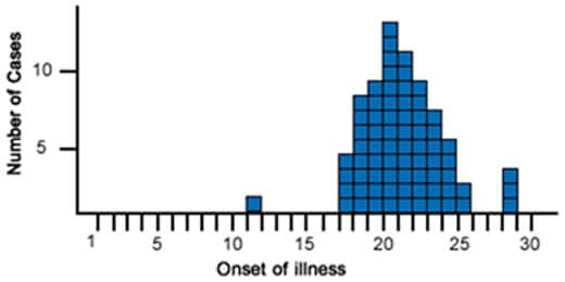
Point Source Outbreak: A sharp rise and fall in cases, indicating a single source of exposure.
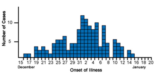
Continuous Common Source Outbreak: A gradual, flat curve indicating ongoing exposure to the same source.
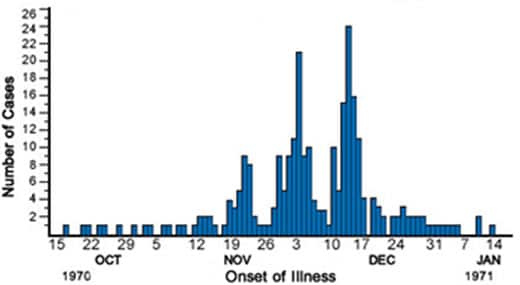
Propagated Outbreak: Multiple peaks, showing successive waves of person-to-person transmission.

How do public health officials use epi curves?

Epi curves help public health officials understand the timing, spread, and source of an outbreak. They are used to track disease progression, assess intervention effectiveness, and predict future cases.

What are the limitations of epi curves?

Some limitations of epi curves include data quality issues, challenges in interpretation without additional data, and complexity in cases where multiple sources or transmission methods are involved in an outbreak.

What Are Epi Curves?

An epidemic curve (epi curve) is a type of histogram that visualizes the number of new cases of a disease or health condition over time. The x-axis represents time (e.g., days, weeks, or months), while the y-axis shows the number of cases. By tracking cases across time, epi curves help epidemiologists and public health officials understand how an outbreak evolves, allowing them to identify its potential source, mode of transmission, and peak period.

Epi curves are especially useful during infectious disease outbreaks but can also be applied to other public health events, such as foodborne illnesses, chemical exposures, or natural disasters.

Why Are Epi Curves Important?

Epi curves provide several key insights during an outbreak:

Understanding the Timing of an Outbreak: Epi curves illustrate when cases start, peak, and decline, allowing public health officials to identify the onset of an outbreak and how quickly it progresses.
Determining the Source of Exposure: By examining the shape of the curve, epidemiologists can infer whether the outbreak was caused by a single source (point source), continuous exposure, or propagated transmission (person-to-person spread).
Assessing the Effectiveness of Interventions: Public health interventions, such as quarantine measures, vaccinations, or public education campaigns, can alter the shape of the epi curve. A drop in cases after an intervention indicates its potential success.
Predicting Future Cases: Based on the pattern of the curve, public health professionals can estimate how many more cases may occur and how long the outbreak will last.

Components of an Epi Curve

To interpret an epi curve effectively, it’s essential to understand its core components:

X-Axis (Time): The horizontal axis represents time, typically in units like days, weeks, or months, depending on the outbreak’s duration. This axis shows when cases occurred. It should be noted that as the dynamics of an outbreak change, it’s possible that the best time scale for representing that outbreak may also change to better inform operations or the public.
Y-Axis (Number of Cases): The vertical axis shows the number of cases (or other health events) occurring within each time period.
Bars or Columns: Each bar on the graph represents the number of new cases during a specific time period. By looking at the height of the bars, epidemiologists can assess the rise and fall of cases.

Example of an Epi Curve in Action

Imagine an outbreak of a foodborne illness, such as salmonella. The epi curve shows when the first cases were reported and tracks the spread of the illness over time. If the cases spike quickly and then decline just as rapidly, it suggests a point-source outbreak, where all individuals were exposed to the pathogen around the same time (e.g., at a contaminated restaurant who got a bad batch of an ingredient). If cases rise more gradually and stay elevated over a longer period, it may indicate ongoing exposure or person-to-person transmission.

Types of Epi Curves

There are several types of epi curves, each representing different outbreak patterns:

Point Source Outbreak: In a point source outbreak, individuals are exposed to the same source of infection at the
An example of a Point Source Outbreak Epi Curve. (Source: CDC)

same time. The epi curve for a point source outbreak typically shows a sharp rise in cases, followed by a gradual decline. An example would be a food poisoning incident where individuals who ate contaminated food develop symptoms within a few hours or days of exposure.

Continuous Common Source Outbreak: In a continuous common source outbreak, individuals are exposed to the infectious agent over a longer period.
An example of a Continuous Common Source Outbreak Epi Curve. (Source: CDC)

The epi curve tends to be flat, as new cases continue to occur as long as the source remains active. For example, contaminated water in a community may cause new cases of illness to appear regularly until the water source is cleaned or shut down.

Propagated Outbreak: In a propagated outbreak, the disease spreads from person to person, leading to successive “waves” of cases.
An example of a Propagated Outbreak Epi Curve. (Source: CDC)

The epi curve for a propagated outbreak shows multiple peaks, each corresponding to a new generation of transmission. This pattern is commonly seen with highly contagious diseases like measles or the flu.

Visual Comparison of Epi Curves

Point Source Curve: The curve rises sharply and then falls, resembling a peak. This suggests that many people were exposed at once, and the outbreak was brief.
Continuous Source Curve: The curve is more gradual and flat, as new cases arise over time due to ongoing exposure.
Propagated Curve: The curve shows a series of peaks, with each new peak representing a subsequent wave of infections due to human-to-human transmission.

How to Interpret an Epi Curve

Interpreting an epi curve requires considering several factors:

Shape of the Curve: The shape of the epi curve provides clues about the type of outbreak. A sharp peak suggests a point source, while a flat curve with sustained cases suggests continuous exposure. Multiple peaks suggest propagated transmission.
Time of Onset: The date when cases first appear on the curve indicates when the outbreak likely started. For infectious diseases, this information helps estimate the incubation period, which is the time between exposure and the onset of symptoms.
Peak of the Outbreak: The highest point on the curve represents the peak of the outbreak, where the most cases occurred in a given period. Identifying the peak helps gauge when the outbreak was at its worst and when it might start to decline.
End of the Outbreak: The point where the curve returns to baseline (i.e., when no more new cases are reported) indicates the end of the outbreak. If the curve doesn’t return to baseline quickly, it may signal ongoing transmission or incomplete containment efforts.

The Role of Epi Curves in Outbreak Investigations

Epi curves are indispensable in the field of outbreak investigations. When a disease outbreak occurs, public health officials need a rapid and reliable way to understand how the outbreak is unfolding and where to intervene. Epi curves offer a real-time visualization of case progression, helping investigators to:

Determine the source of infection: By pinpointing the earliest cases and understanding the shape of the curve, epidemiologists can trace the source of exposure (e.g., contaminated food, infected individuals, or environmental hazards).
Identify the mode of transmission: The shape of the curve can reveal whether the disease is spreading through contaminated sources (point or continuous exposure) or through person-to-person contact (propagated transmission).
Evaluate the impact of interventions: As public health interventions, such as vaccination campaigns or quarantine measures, are implemented, the shape of the epi curve may change, indicating the effectiveness of these strategies.

Limitations of Epi Curves

While epi curves are valuable tools in public health, they have some limitations:

Data Quality: The accuracy of an epi curve depends on the completeness and timeliness of the data. Delays in reporting or incomplete case data can lead to a distorted view of the outbreak’s progression. During normal outbreak investigations and response, data quality will often be uncertain, so using best practices and what is available is generally accepted.
Interpretation: Epi curves alone cannot provide conclusive evidence about the cause of an outbreak. Additional epidemiological data, such as patient interviews, laboratory tests, and environmental assessments, are often needed to confirm the source of the outbreak.
Complex Outbreaks: In outbreaks with multiple sources or varying transmission modes, the epi curve may be difficult to interpret, as it might show overlapping patterns that don’t fit neatly into the standard outbreak types (point source, continuous, propagated).

Conclusion

An epidemic curve is a vital tool in epidemiology, providing a visual representation of how a disease outbreak progresses over time. By tracking the number of new cases across time intervals, public health professionals can identify the source of the outbreak, determine how the disease is spreading, and assess the effectiveness of interventions.

Although epi curves cannot explain everything about an outbreak, they are an essential starting point for public health investigations and are often used in conjunction with other epidemiological tools to uncover the root causes of disease outbreaks and inform public health actions.

Humanities Moment

The featured image for this installment of Epi Explained is Winter’s Cabin at the Curve by Birge Harrison (American, 1854–1929). Lovell Birge Harrison was an American landscape and genre painter, teacher, and writer, known for his advocacy of Tonalism. Born in Philadelphia, he studied under Thomas Eakins, Carolus-Duran, and at the École des Beaux-Arts, becoming one of the first American artists to have work purchased by the French government. Harrison, influenced by atmospheric painting techniques, became a leader of the Tonalist school after moving to Woodstock, New York, where he founded a painting school. He was a celebrated artist and writer, receiving numerous accolades and publishing influential works on landscape painting, emphasizing honest observation of nature.

Thank you for reading this Epi Explained. If you’d like to learn more about epidemiology, public health, programming or other key topics, please check out more of our website!

Community trials

In this tutorial, we will cover community trials, a type of experimental study design used in public health. Community trials are conducted at the community level rather than with individuals and are often used to evaluate the impact of public health interventions aimed at improving health outcomes across large populations. Understanding community trials is important for the Certified in Public Health (CPH) exam.

By the end of this tutorial, you will understand how community trials are designed, their strengths and limitations, and when they are used in public health research. We will also include practice questions to help reinforce your understanding.

1. Introduction to Experimental Studies

Experimental studies are designed to test the effectiveness of interventions by assigning individuals or groups to receive an intervention or a control. Unlike observational studies, experimental studies allow researchers to control variables and draw stronger conclusions about cause-and-effect relationships. A community trial is a type of experimental study where entire communities, rather than individuals, are the unit of analysis.

2. What Are Community Trials?

A community trial, also known as a community intervention trial or field trial, is an experimental study where entire communities or groups (rather than individuals) are assigned to receive an intervention. Community trials are used to evaluate the effectiveness of public health programs and interventions aimed at improving health outcomes on a large scale.

2.1 Definition of Community Trials

In a community trial, entire communities are randomly assigned to either receive a public health intervention (such as a health promotion program or environmental change) or to serve as a control (receiving no intervention or a standard intervention). The effects of the intervention are measured by comparing health outcomes between the intervention and control communities.

2.2 Key Features of Community Trials

Unit of analysis: Communities or groups, rather than individuals, are the unit of analysis.
Randomization: Communities are often randomly assigned to intervention or control groups to reduce bias.
Public health focus: Community trials often aim to assess the effectiveness of interventions such as education campaigns, vaccination programs, or environmental health initiatives.
Long-term follow-up: Community trials often require extended follow-up to assess the sustainability and long-term effects of interventions.

3. Steps in Conducting a Community Trial

Community trials follow a systematic process to ensure the validity and reliability of the results. Here are the key steps involved:

Select the communities: Choose communities or groups that are similar in terms of demographics and health characteristics to ensure comparability.
Randomize communities: Assign communities randomly to either the intervention group or the control group to minimize bias and ensure that differences in outcomes can be attributed to the intervention.
Implement the intervention: Deliver the public health intervention to the intervention communities, such as health education programs, policy changes, or environmental modifications.
Monitor and follow up: Collect data on health outcomes and other relevant measures in both the intervention and control communities over time.
Analyze the data: Compare outcomes between the intervention and control communities to assess the effectiveness of the intervention.
Report the results: Publish the findings, highlighting any successes, challenges, and limitations of the trial.

4. Advantages of Community Trials

Community trials offer several advantages, particularly when assessing public health interventions:

Real-world application: Community trials are conducted in real-world settings, allowing researchers to evaluate the effectiveness of interventions under realistic conditions.
Large-scale impact: Since community trials target entire populations, they can assess the effectiveness of interventions aimed at improving public health on a large scale.
Generalizable results: Because they are conducted in community settings, the results are often (but not always!) more generalizable to the broader population.
Public health relevance: Community trials often assess interventions that address important public health issues, such as smoking cessation, obesity prevention, or infectious disease control.

5. Limitations of Community Trials

Despite their strengths, community trials also have limitations:

Expensive and time-consuming: Community trials require significant resources, as they involve large populations and long-term follow-up.
Complex logistics: Implementing and monitoring interventions at the community level can be challenging, especially in diverse or hard-to-reach populations.
Contamination risk: There is a risk of contamination, where members of the control group may be exposed to the intervention, which can affect the study’s outcomes.
Ethical concerns: Community trials may raise ethical issues, particularly if the intervention could benefit the control group but is withheld during the study.

6. When to Use Community Trials

Community trials are best used when the goal is to evaluate the impact of public health interventions on a large scale. They are commonly used in the following situations:

Public health campaigns: To assess the effectiveness of health promotion campaigns, such as smoking cessation, safe drinking water initiatives, or vaccination drives.
Policy changes: To evaluate the impact of policy changes on health outcomes, such as new laws banning smoking in public places or policies promoting healthier school lunches.
Environmental interventions: To assess the effectiveness of interventions that alter the physical environment, such as creating safe walking paths, improving sanitation, or reducing pollution.

Example: A community trial might be used to evaluate the impact of a new smoking cessation program by comparing smoking rates between communities that receive the program and those that do not.

7. Practice Questions

Let’s test your understanding of community trials with these practice questions. Try answering them before checking the solutions.

Question 1:

A study randomly assigns 10 communities to receive a health education program aimed at reducing obesity, while 10 other communities do not receive the program. What type of study design is this?

Answer 1:

Answer, click to reveal

This is a community trial because entire communities, rather than individuals, are assigned to receive the intervention (health education program).

Question 2:

What is one key advantage of community trials over individual-level trials?

Answer 2:

Answer, click to reveal

One key advantage of community trials is that they evaluate interventions at the population level, providing insights into the effectiveness of public health programs on a larger scale.

Question 3:

Why might a community trial be difficult to implement in practice?

Answer 3:

Answer, click to reveal

Community trials can be difficult to implement due to the complex logistics involved in managing large populations, ensuring compliance with the intervention, and preventing contamination between intervention and control groups. Likewise, in some scenarios, ethical concerns may make such a study format unfeasible.

8. Conclusion

Community trials are an important experimental study design in public health research. By targeting entire populations, they allow researchers to evaluate the effectiveness of public health interventions on a large scale. However, they can be resource-intensive and logistically complex, and one has to be aware of potential ethical limitations of this approach.

Remember:

Community trials assess interventions at the community level, making them useful for evaluating public health campaigns and policies.
They offer real-world application and results that are generalizable to larger populations.
They can be expensive and time-consuming but provide valuable insights into the impact of public health interventions on population health.

Final Tip for the CPH Exam:

Be sure to understand the differences between community trials and individual-level trials, as well as the unique advantages and limitations of each. Practice identifying scenarios where community trials are the most appropriate study design for evaluating public health interventions.

Humanities Moment

The featured image for this article is House and factories as seen on the edge of a community (1849) by James Fuller Queen (American, 1820-1886). James Fuller Queen was a prominent Philadelphia lithographer known for his detailed chromolithographs and contributions to Civil War-era fundraising prints. His extensive output and lifelong dedication to the trade was clear, though less well known was his many years of community service, and the fact left a significant estate at his death in 1886 to his community.

Randomized controlled trials

In this tutorial, we will explore randomized controlled trials (RCTs), a key type of experimental study design. RCTs are considered the gold standard for determining the effectiveness of interventions and are widely used in public health and clinical research. Understanding how RCTs are designed and conducted is very useful for the Certified in Public Health (CPH) exam.

By the end of this tutorial, you will understand the design, advantages, and limitations of randomized controlled trials, as well as when and how they are used in public health research. We will also include practice questions to help reinforce your knowledge.

1. Introduction to Experimental Studies

Experimental studies differ from observational studies in that the investigator actively intervenes by assigning participants to different treatment or exposure groups. The goal is to assess the effects of specific interventions or treatments on outcomes. The most well-known type of experimental study is the randomized controlled trial (RCT).

2. What Are Randomized Controlled Trials?

A randomized controlled trial (RCT) is a type of experimental study in which participants are randomly assigned to either the intervention group (receiving the treatment) or the control group (receiving a placebo or standard care). RCTs are designed to minimize bias and provide the most reliable evidence about the effectiveness of interventions.

2.1 Definition of RCTs

In an RCT, participants are randomly allocated to one of two or more groups to receive different interventions. The random assignment ensures that any differences in outcomes between groups can be attributed to the intervention itself, rather than other confounding factors.

2.2 Key Features of RCTs

Randomization: Participants are randomly assigned to intervention or control groups to reduce selection bias.
Control Group: The control group may receive a placebo, no treatment, or the standard of care, allowing for comparison with the intervention group.
Blinding: In many RCTs, participants, healthcare providers, and/or researchers are “blinded” (i.e., unaware of which group participants are in) to reduce bias.
Follow-up: Participants are followed over time to measure outcomes related to the intervention.

3. Steps in Conducting an RCT

RCTs follow a systematic process to ensure the validity and reliability of the results. Here are the key steps involved:

Design the study: Define the research question, study population, and outcomes of interest. Develop inclusion and exclusion criteria for participants.
Randomize participants: Assign participants randomly to the intervention or control group. This can be done using computer-generated randomization or other randomization methods.
Implement the intervention: Administer the intervention to the experimental group and ensure that the control group receives a placebo or standard care.
Blinding (if applicable): Implement blinding to prevent bias. In a double-blind study, neither participants nor researchers know who is in the intervention group.
Follow-up: Collect data on outcomes over a specified follow-up period to assess the effects of the intervention.
Analyze the data: Compare the outcomes between the intervention and control groups using statistical methods to determine the effectiveness of the intervention.
Report the results: Publish the findings, including any adverse effects or limitations of the study.

4. Advantages of Randomized Controlled Trials

RCTs offer several advantages that make them the gold standard in research:

Minimizes bias: Randomization and blinding reduce selection and information bias, ensuring that the results are reliable and unbiased.
Strongest evidence for causality: By controlling the allocation of interventions, RCTs provide the most direct evidence of a causal relationship between an intervention and an outcome.
Controlled comparison: RCTs allow for a direct comparison between intervention and control groups, enabling researchers to determine the effectiveness of the intervention.
Generalizable results: When conducted with a representative sample, RCTs can provide results that are generalizable to larger populations.

5. Limitations of Randomized Controlled Trials

Despite their strengths, RCTs have several limitations:

Costly and time-consuming: RCTs require significant resources, including funding, personnel, and time, making them expensive to conduct.
Ethical concerns: It may be unethical to withhold a potentially beneficial treatment from the control group, or to expose participants to harmful interventions.
Not always feasible: For rare diseases or long-term outcomes, it may not be practical to conduct an RCT due to the large sample size or long follow-up required.
Limited external validity: Results from RCTs may not be generalizable to the wider population if the study sample is not representative.

6. When to Use Randomized Controlled Trials

RCTs are the preferred study design when the goal is to evaluate the efficacy of a specific intervention or treatment. They are commonly used in the following situations:

Clinical trials: RCTs are widely used to test new medications, treatments, or medical devices for safety and efficacy.
Public health interventions: RCTs can be used to evaluate the impact of public health programs, such as smoking cessation programs or vaccination campaigns.
Behavioral interventions: RCTs are used to assess the effectiveness of behavioral interventions, such as diet or exercise programs.

Example: A randomized controlled trial is conducted to assess the effectiveness of a new drug in reducing blood pressure. Participants are randomly assigned to receive either the new drug or a placebo, and their blood pressure levels are monitored over time to assess the drug’s efficacy.

7. Practice Questions

Let’s reinforce your understanding with some practice questions. Try answering these before checking the solutions.

Question 1:

A study randomly assigns 500 participants to either a new diet program or a standard diet. The participants’ weight loss is tracked over 12 months. What type of study design is this?

Answer 1:

Answer, click to reveal

This is a randomized controlled trial (RCT) because participants are randomly assigned to intervention (new diet) and control (standard diet) groups, and their outcomes (weight loss) are measured over time.

Question 2:

What is one major advantage of an RCT over observational studies?

Answer 2:

Answer, click to reveal

One major advantage of RCTs is that they minimize bias by randomly assigning participants to intervention or control groups, reducing the influence of confounding variables.

Question 3:

Why might conducting an RCT be considered unethical in some cases?

Answer 3:

Answer, click to reveal

Conducting an RCT may be considered unethical if it involves withholding a potentially beneficial treatment from the control group or exposing participants to harmful interventions.

8. Conclusion

Randomized controlled trials (RCTs) are the most rigorous study design for evaluating the effectiveness of interventions. By randomly assigning participants to different treatment groups, RCTs reduce bias and provide strong evidence for causality. However, they can be costly, time-consuming, and sometimes unethical to conduct.

Remember:

RCTs involve random assignment to intervention and control groups, making them the gold standard for determining causality.
They are best suited for clinical trials and public health interventions where the goal is to evaluate the efficacy of a specific treatment or program.
RCTs can be expensive and time-consuming but offer the most reliable results when conducted properly.

Final Tip for the CPH Exam:

Make sure you understand the key features of randomized controlled trials, their advantages and limitations, and how they differ from observational studies. Practice identifying scenarios where RCTs are the appropriate study design for evaluating interventions, and read at least a few published studies that use RCTs and ask yourself what other studies could have been used in ideal conditions, and why.

Humanities Moment

The featured image for this article is Cibotium regale (1854-1896) by Charles Antoine Lemaire (French, 1800-1871). Lemaire was a French botanist and botanical author, known for his work on Cactaceae and for editing influential gardening journals. Despite his extensive contributions to botanical literature, including naming the genus Schlumbergera, he lived in poverty and never published a major work on cacti.

Epi Explained: What are Non-Pharmaceutical Interventions (NPIs)?

Non-Pharmaceutical Interventions (NPIs) are actions, apart from medical treatments like vaccines and medications, that individuals and communities can take to help slow the spread of contagious diseases. NPIs are crucial during outbreaks and pandemics, especially when vaccines or treatments are unavailable, limited, or ineffective against the disease. These interventions include strategies such as social distancing, mask-wearing, quarantine, isolation, travel restrictions, and personal hygiene practices, all designed to reduce human-to-human transmission.

In this EpiExplained, we’ll cover the various types of NPIs, factors to consider when implementing them, the concept of social fatigue, and historical examples of NPIs in action.

Key Questions

What are Non-Pharmaceutical Interventions (NPIs)?

Non-Pharmaceutical Interventions (NPIs) are measures that individuals and communities can implement to reduce the spread of infectious diseases without the use of medical treatments such as vaccines or medications. Examples include hand hygiene, social distancing, mask-wearing, and quarantines.

Why are NPIs important during an outbreak?

NPIs are critical in controlling disease transmission, especially when vaccines or treatments are not yet available, or during the early stages of an outbreak. They help reduce the number of cases, protect healthcare systems, and limit the spread of the disease.

What factors influence the success of NPIs?

The success of NPIs depends on factors such as timing, public compliance, economic impacts, and the effectiveness of communication from health authorities. Cultural attitudes and access to resources also play a role in how well NPIs are adopted.

Social fatigue occurs when individuals become tired or frustrated with prolonged restrictions, such as social distancing or mask-wearing. This can lead to reduced compliance and increased disease transmission, making it important to manage public expectations and offer support.

Can NPIs completely stop an outbreak?

NPIs can slow the spread of a disease and reduce its impact, but they are often most effective when used in combination with other public health measures, such as testing, contact tracing, and vaccination campaigns once available.

What are Non-Pharmaceutical Interventions (NPIs)?

Non-Pharmaceutical Interventions (NPIs) are measures that reduce the spread of infectious diseases without the use of pharmaceuticals, such as vaccines or antiviral medications. These interventions are often implemented to delay the spread of a disease, reduce the peak burden on healthcare systems, and protect high-risk populations. NPIs are particularly important during the early stages of an outbreak when medical countermeasures may not yet be available or widely distributed.

NPIs are not one-size-fits-all solutions. Their effectiveness depends on the type of disease, how it spreads, the population’s characteristics, and the timing and stringency of the interventions. In this article, we’ll explore the different categories of NPIs, key considerations for implementing them, their societal impact, and examples of their use throughout history.

Categories of NPIs

NPIs are generally categorized into three main types: personal protective measures, community-level measures, and environmental measures. Each category targets a different level of disease prevention, from individual actions to widespread societal changes.

1. Personal Protective Measures

Personal NPIs are actions that individuals can take to reduce their risk of contracting or spreading a disease. These are the first line of defense and are typically the most straightforward to implement, although their effectiveness can vary based on individual compliance.

Key Personal NPIs:

Hand Hygiene: Frequent handwashing with soap and water, or using alcohol-based hand sanitizers, is one of the simplest and most effective ways to prevent disease transmission, especially for respiratory and gastrointestinal infections.
Respiratory Etiquette: Covering coughs and sneezes with a tissue or the inside of the elbow reduces the spread of droplets that may carry viruses or bacteria.
Face Masks: Wearing masks, particularly in crowded or enclosed spaces, can help reduce the transmission of respiratory droplets and protect both the wearer and others.
Self-Isolation: Individuals who are symptomatic or have been exposed to a known case of the disease can self-isolate to prevent spreading it to others.

Effectiveness of Personal NPIs:

Personal NPIs rely heavily on individual compliance and can be influenced by public perception, education, and access to resources. For example, proper mask-wearing requires both the availability of masks and correct use.

2. Community-Level Measures

Community NPIs involve larger-scale actions that affect groups of people or entire communities. These measures are usually coordinated by public health authorities or governments and aim to reduce opportunities for close contact and large gatherings, where transmission can easily occur.

Key Community-Level NPIs:

Social Distancing: Maintaining physical space between individuals (typically 6 feet or more) reduces the likelihood of transmitting infectious diseases, particularly airborne or droplet-spread pathogens.
Quarantine and Isolation: Quarantine separates individuals who have been exposed to a disease but are not yet symptomatic, while isolation separates those who are already sick from healthy individuals.
School Closures: Temporarily closing schools can help reduce the spread of infections among children, who are often efficient disease transmitters. School closures also reduce transmission between households.
Remote Work Policies: Encouraging or mandating remote work for non-essential workers reduces the number of people commuting and congregating in workplaces, which helps lower transmission rates.
Event and Gathering Restrictions: Limiting the size of public gatherings, or canceling mass events, can prevent large-scale outbreaks, particularly in enclosed or crowded environments.
Travel Restrictions and Border Controls: Restricting non-essential travel and implementing health checks at borders can slow the spread of diseases, especially those that may be imported from other regions. This can include closing off international borders, provincial borders, or sometimes even small scale communities. This is often seen as a last option due to its impact on the communities in question, and referred to as Cordon Sanitare (French: sanitary cordon).

3. Environmental Measures

Environmental NPIs focus on modifying physical spaces to reduce the spread of disease. These interventions often involve changes in infrastructure or environmental sanitation to limit transmission in shared environments.

Key Environmental NPIs:

Enhanced Cleaning and Disinfection: Increasing the frequency of cleaning and disinfecting high-touch surfaces (e.g., door handles, elevator buttons) in public spaces, schools, workplaces, and transportation systems can reduce the transmission of pathogens.
Ventilation Improvements: Improving indoor ventilation by opening windows, using air filtration systems, or modifying heating, ventilation, and air conditioning (HVAC) systems can help disperse infectious particles and lower the risk of airborne transmission.
Physical Barriers: Installing physical barriers, such as plexiglass shields, in areas where maintaining physical distance is difficult (e.g., retail counters) can help prevent direct contact between individuals.
Building Modifications: Creating one-way pedestrian traffic flows, widening walkways, and redesigning shared spaces can reduce close contact in places where people congregate.

Factors to Consider When Implementing NPIs

While NPIs are essential tools in controlling the spread of infectious diseases, their implementation requires careful consideration of various factors to ensure their effectiveness and minimize unintended consequences.

1. Timing and Stage of the Outbreak

The timing of NPI implementation is critical. Early intervention often yields the best results in controlling disease spread. However, if implemented too late, NPIs may not significantly affect the outbreak’s trajectory.

Early Implementation: Introducing NPIs at the beginning of an outbreak can “flatten the curve,” slowing the disease’s spread and preventing healthcare systems from being overwhelmed.
Delayed Implementation: Waiting too long to implement NPIs can lead to rapid disease transmission and an explosive increase in cases, making it harder to control the outbreak.

2. Compliance and Public Perception

The success of NPIs depends largely on public adherence. Factors that influence compliance include:

Public Trust: Trust in public health authorities and government recommendations is crucial. Clear, consistent, and transparent communication fosters compliance. It should be noted that often times, the public views the actions of any government agency as “The Government”, so being cognizant of not only what your agency is doing, but of those who can be grouped in with you is essential. Often times, being able to have good relationships with community leaders can help increase public trust, but takes time and should be prioritized in a so-called Blue Sky (normal/day-to-day) environment, and not be undertaken only after something has occurred. Failure to do so can often reinforce the image of “outsiders” coming in to tell communities what to do and taking away rights, even if the intent is purely to save lives and decrease impacts of disease.
Cultural Norms: Cultural attitudes toward certain interventions, like mask-wearing or social distancing, can affect how well NPIs are adopted. In some cultures, wearing masks in public has long been normalized, while in others, it may be viewed with skepticism or resistance.
Access to Resources: Ensuring that individuals have the necessary resources to comply with NPIs is vital. For instance, hand hygiene requires access to clean water, soap, or hand sanitizers, and mask mandates require widespread availability of masks.

NPIs, especially community-level and environmental interventions, often have economic and social implications that need to be weighed against their public health benefits.

Economic Impact: Measures like business closures, travel bans, and remote work mandates can have significant economic consequences, particularly for industries reliant on physical interaction, such as hospitality, tourism, and retail. However, this should always be considered alongside the very real cost in human lives of prioritizing business interests over appropriate NPI implementation.
Equity Issues: Some NPIs may disproportionately affect certain populations, particularly low-income communities, essential workers, and those without access to healthcare or paid sick leave. Governments must ensure that vulnerable groups are supported during NPI implementation, such as providing financial aid, social services, adequate protective equipment, etc.
Educational Disruptions: School closures, while effective in controlling outbreaks, can disrupt learning, particularly for students in disadvantaged communities who may lack access to online education or resources.

One of the key challenges of long-term NPI implementation is social fatigue. As NPIs, such as social distancing, mask-wearing, and travel restrictions, remain in place for extended periods, individuals and communities may experience psychological and emotional fatigue. This can lead to reduced compliance, even if the measures are still necessary to control disease transmission.

Duration of Restrictions: The longer NPIs are in place, the more likely people are to feel frustrated, anxious, and isolated, leading to non-compliance. People may begin to disregard recommendations, such as avoiding large gatherings, as they become fatigued by the restrictions.
Lack of Clear Communication: When public health messaging is inconsistent or unclear, it can lead to confusion and reduce public trust in the measures. People may question the effectiveness or necessity of NPIs, especially if they do not see immediate results. Clear Communication should also not be confused with keeping to only one message, especially if the information is out of date or ineffective. Acknowledging a changing landscape and taking ownership of decisions, and communicating that as well, can increase public trust and adherence.
Social and Economic Pressures: Prolonged NPIs can strain social networks, economic livelihoods, and mental health. Job losses, financial stress, and isolation from loved ones contribute to social fatigue and increase the desire to return to normal activities.
Perceived Ineffectiveness: If the disease persists despite NPIs, some individuals may view the interventions as ineffective and stop following them, even if those measures are still critical to controlling the outbreak.

Targeted Messaging: Clear, consistent, and evidence-based communication about the importance of NPIs is essential. Public health authorities should explain the rationale behind interventions, update the public regularly, and provide a timeline or benchmarks for lifting restrictions.
Balancing Restrictions with Flexibility: Authorities should seek a balance between necessary restrictions and social flexibility. For example, allowing outdoor activities with safety measures in place can provide individuals with a sense of normalcy without compromising public health.
Mental Health Support: Offering mental health services, promoting community engagement (virtually or safely in-person), and encouraging physical activity can help alleviate some of the emotional and psychological burdens of prolonged NPIs.

Historical Examples of NPIs

Throughout history, NPIs have been used to combat infectious diseases long before modern medicine developed effective vaccines or treatments. Here are some notable examples of NPIs in action:

1. The 1918 Influenza Pandemic

During the 1918 influenza pandemic, also known as the Spanish flu (despite having an origination point in Kansas, United States), NPIs such as social distancing, quarantines, and the use of masks were implemented in many cities worldwide to slow the spread of the virus. The pandemic, which killed an estimated 50 million people globally, showcased both the strengths and limitations of NPIs.

Success Stories: Cities like St. Louis implemented strict social distancing measures early in the outbreak and were able to reduce peak mortality rates significantly. Public health campaigns promoted mask-wearing, and schools, theaters, and businesses were temporarily closed.
Challenges: Other cities, such as Philadelphia, delayed the implementation of NPIs, leading to devastating surges in cases and overwhelming healthcare systems.

2. The SARS Outbreak of 2003

The SARS (Severe Acute Respiratory Syndrome) outbreak in 2003 demonstrated the importance of NPIs in containing a highly contagious and deadly respiratory virus. SARS spread to 26 countries, but through aggressive implementation of NPIs, including isolation, quarantine, travel restrictions, and contact tracing, the outbreak was largely contained within a few months.

Quarantine and Isolation: Quarantining suspected cases and isolating confirmed patients were central to controlling SARS. The rapid identification and isolation of cases prevented widespread community transmission.
Global Coordination: Countries worked together to implement NPIs at a global level, particularly in restricting travel and screening individuals at borders, which limited the spread of the virus across borders.

3. The COVID-19 Pandemic (2020-Present)

The COVID-19 pandemic is perhaps the most well-known example of NPIs being deployed on a global scale. With no available vaccine or specific treatment in the early months of the pandemic, NPIs became the primary strategy for controlling the spread of the SARS-CoV-2 virus.

Widespread Lockdowns: Countries around the world implemented varying levels of lockdowns, including school and business closures, stay-at-home orders, and bans on public gatherings. These measures helped reduce transmission, but also had significant social and economic impacts.
Mask Mandates: The widespread use of masks, particularly in indoor and crowded settings, was promoted as an essential NPI to reduce airborne transmission of the virus. Public health messaging and government mandates varied widely between regions, leading to differences in compliance.
Travel Bans and Quarantines: Many countries implemented strict travel restrictions, including mandatory quarantine for incoming travelers and bans on non-essential international travel, which helped limit cross-border transmission.

Conclusion

Non-Pharmaceutical Interventions (NPIs) are critical tools in the control of infectious disease outbreaks, especially when vaccines or treatments are unavailable or insufficient. From personal actions like hand hygiene and mask-wearing to community-wide measures like social distancing, quarantine, and travel restrictions, NPIs have been proven effective in reducing transmission.

However, implementing NPIs requires careful consideration of timing, compliance, social impacts, and other consequences. Long-term reliance on NPIs can also lead to social fatigue, making it essential for public health officials to balance restrictions with maintaining public trust and keeping the public adequately engaged and informed.

Historically, NPIs have been used successfully to combat pandemics like the 1918 influenza, SARS in 2003, and COVID-19. Their continued relevance highlights the importance of preparedness and public health infrastructure in addressing future outbreaks.

Humanities Moment

The featured image for this Epi Explained is The Hand Washing (Allegory of Water) by Bernhard Keil (Danish, 1624-1687). Bernhard Keil, also known as Keyl, was a Danish Baroque painter born in Helsingør who became a pupil of Rembrandt. After studying with Danish painter Morten Steenwinkel and later working in Amsterdam, Keil established his own workshop before traveling to Rome in 1656, where he worked until his death in 1687. His work was influenced by Jan Lievens, and he, in turn, influenced artists such as Pietro Bellotti, Antonio Cifrondi, and Giacomo Francesco Cipper. Keil also worked in Bergamo and Venice during his career.

Thank you for reading this very extended Epi Explained article. If you’d like to check out our other topics, a browse through our website would be greatly appreciated!

Cross-sectional studies

In this tutorial, we will focus on a commonly used study design in epidemiology: cross-sectional studies. Cross-sectional studies are useful for understanding the prevalence of diseases or health-related factors at a specific point in time. This design is occasionally used in public health research and is essential knowledge for the Certified in Public Health (CPH) exam.

By the end of this tutorial, you will understand how cross-sectional studies are conducted, when to use them, and their advantages and limitations. We will also provide practice questions to help reinforce your understanding.

1. Introduction to Analytical Studies

Analytical studies are designed to test hypotheses about associations between risk factors and health outcomes. Cross-sectional studies, although often considered descriptive, can also be analytical when they are used to assess the relationship between an exposure and an outcome at a specific point in time.

2. What Are Cross-Sectional Studies?

A cross-sectional study is an observational study that analyzes data from a population at a specific point in time. It is used to assess the prevalence of a disease or risk factor within a population and to explore associations between exposure and outcome.

2.1 Definition of Cross-Sectional Studies

In a cross-sectional study, data are collected at a single point in time from a sample that represents a population. The study provides a snapshot of the population’s health status, exposure levels, and outcomes at that time.

2.2 Key Features of Cross-Sectional Studies

Measures both exposure and outcome at the same point in time.
Data are collected from a sample that is representative of the population.
Prevalence (the proportion of individuals with a disease or outcome) is the main measure of interest.
Commonly used to assess health behaviors, risk factors, and disease prevalence in populations.

3. When to Use Cross-Sectional Studies

Cross-sectional studies are useful in the following situations:

When the goal is to determine the prevalence of a health outcome or behavior in a population.
When studying multiple outcomes or exposures at the same time.
When conducting surveys or health assessments to guide public health policy or interventions.

Example: A cross-sectional study could be used to assess the prevalence of smoking and its association with respiratory disease in a population by collecting data on smoking habits and lung health at a single point in time.

4. Advantages of Cross-Sectional Studies

Cross-sectional studies offer several advantages:

Quick and cost-effective: Since data are collected at one point in time, cross-sectional studies are faster and less expensive than longitudinal studies.
Useful for assessing prevalence: They are ideal for estimating the prevalence of health outcomes, diseases, or behaviors within a population.
Good for generating hypotheses: Cross-sectional studies can identify potential associations between risk factors and outcomes that can be explored further in more rigorous studies.
Multiple outcomes and exposures: They allow for the simultaneous measurement of various outcomes and exposures in a population.

5. Limitations of Cross-Sectional Studies

Despite their usefulness, cross-sectional studies have limitations:

Cannot establish causality: Since exposure and outcome are measured at the same time, it is difficult to determine whether the exposure preceded the outcome.
Risk of confounding: Other factors not accounted for in the study could influence the association between exposure and outcome.
Prone to prevalence-incidence bias: Cross-sectional studies measure existing cases of disease (prevalence) rather than new cases (incidence), which may not reflect the true rate of disease development.

6. Comparing Cross-Sectional Studies with Other Study Designs

Cross-sectional studies differ from other analytical study designs, such as cohort studies and case-control studies, in several ways:

Cross-Sectional Studies: Measure exposure and outcome at the same point in time. Useful for estimating prevalence but cannot establish temporal relationships between exposure and outcome.
Cohort Studies: Follow a group over time, measuring exposure before the outcome occurs, allowing researchers to establish a temporal relationship and calculate incidence rates.
Case-Control Studies: Start with the outcome (disease) and look back to assess past exposures, which makes them more suitable for studying rare diseases.

Feature	Cross-Sectional Studies	Cohort Studies	Case-Control Studies
Timing	Exposure and outcome measured simultaneously	Exposure measured before outcome	Outcome identified before exposure assessment
Cost and Time	Quick and inexpensive	Time-consuming and costly	Moderately expensive, faster than cohort studies
Ability to Establish Causality	Cannot establish causality	Can establish temporal relationships, better for causality	Cannot establish causality

7. Practice Questions

Test your understanding of cross-sectional studies with these practice questions. Try answering them before checking the solutions.

Question 1:

A study collects data on the prevalence of obesity and physical activity in a population at a single point in time. What type of study design is this?

Answer 1:

Answer, click to reveal

This is a cross-sectional study because it measures both obesity and physical activity in the population at one point in time.

Question 2:

What is one key advantage of cross-sectional studies?

Answer 2:

Answer, click to reveal

Cross-sectional studies are quick and cost-effective because they involve collecting data at a single point in time rather than following participants over a long period.

Question 3:

Why are cross-sectional studies unable to establish causality?

Answer 3:

Answer, click to reveal

Cross-sectional studies measure exposure and outcome simultaneously, making it impossible to determine whether the exposure preceded the outcome.

8. Conclusion

Cross-sectional studies are a valuable tool in public health for assessing the prevalence of diseases, health behaviors, and risk factors. While they are limited by their inability to establish causality, they are an efficient and cost-effective method for generating hypotheses and identifying associations between exposures and outcomes.

Remember:

Cross-sectional studies provide a snapshot of a population’s health at a specific point in time.
They are useful for measuring prevalence but cannot establish a temporal relationship between exposure and outcome.
They are quick and inexpensive, making them ideal for large-scale surveys and health assessments.

Final Tip for the CPH Exam:

Make sure you can identify the unique features of cross-sectional studies and understand how they differ from cohort and case-control studies. Practice identifying appropriate scenarios for cross-sectional studies in exam questions, particularly when the goal is to measure prevalence.

Humanities Moment

The featured image for this article is Approach to Venice (1844)by Joseph Mallord William Turner (English, 1775-1851). Turner was a renowned English Romantic painter known for his vivid use of color and dramatic landscapes, especially turbulent seascapes. A private and eccentric figure, he produced thousands of works, greatly influenced landscape painting, and lived reclusively in London until his death in 1851, leaving a lasting legacy in art.