Incidence and prevalence

In this CPH Focus, we’ll dive deep into one of the fundamental topics in public health: measures of disease frequency, specifically incidence and prevalence. Understanding these concepts is crucial for the Certified in Public Health (CPH) exam and serves as a foundation for working in the public health field.

By the end of this tutorial, you’ll have a solid grasp of these epidemiological measures, how they are calculated, and when to use each one. We’ll also include practice questions with answers to help solidify your understanding.

1. Introduction to Epidemiology

Epidemiology is the study of how diseases are distributed across populations and what factors influence their spread. It is often described as the cornerstone of public health, as it provides critical insights that can guide policies, interventions, and research.

2. What are Measures of Disease Frequency?

Measures of disease frequency help public health professionals understand how often diseases occur within populations. These measures give insights into:

How common a disease is (prevalence)
How often new cases arise (incidence)

The two primary measures of disease frequency we’ll focus on are:

Incidence
Prevalence

Each provides different but complementary information about disease dynamics in a population.

3. Understanding Incidence

Incidence refers to the number of new cases of a disease or condition that occur in a specific population during a defined period. It helps public health professionals understand the risk of developing a disease.

3.1 Incidence Rate

The incidence rate is a measure of how quickly new cases of a disease arise in a population over time. It accounts for both the number of new cases and the amount of time that the population is at risk.

Formula for Incidence Rate:

$\text{Incidence Rate} = \frac{\text{Number of New Cases}}{\text{Total Person-Time at Risk}}$

Where:

New Cases: The number of individuals who develop the disease during the specified time period.
Person-Time at Risk: The sum of the time that each individual in the population is at risk of developing the disease.

Example:

In a study of 1,000 people observed for 1 year, 50 new cases of disease X were identified. The incidence rate would be:

$\text{Incidence Rate} = \frac{50}{1,000 \text{ person-years}} = 0.05 \text{ cases per person-year}$

This means that for every 100 people observed for 1 year, 5 would develop disease X.

3.2 Cumulative Incidence

Cumulative Incidence is another way to express incidence, focusing on the proportion of a population that develops the disease over a specific period of time.

Formula for Cumulative Incidence:

$\text{Cumulative Incidence} = \frac{\text{Number of New Cases}}{\text{Total Population at Risk at the Start of the Study}}$

Example:

If 50 people in a population of 1,000 develop disease X over 1 year, the cumulative incidence would be:

$\text{Cumulative Incidence} = \frac{50}{1,000} = 0.05 \text{ or } 5\%$

This indicates that 5% of the population developed the disease during the study period.

Key Points About Incidence:

Incidence focuses on new cases.
It helps determine the risk of contracting a disease.
It is particularly useful for acute conditions or diseases with clear onset.

4. Understanding Prevalence

Prevalence refers to the total number of cases, both new and existing, present in a population at a given time. It gives a snapshot of how widespread a disease is in a population.

4.1 Point Prevalence

Point Prevalence is the proportion of the population that has the disease at a specific point in time.

Formula for Point Prevalence:

$\text{Point Prevalence} = \frac{\text{Number of Existing Cases}}{\text{Total Population at the Same Point in Time}}$

Example:

In a town of 1,000 people, 100 individuals currently have disease Y. The point prevalence would be:

$\text{Point Prevalence} = \frac{100}{1,000} = 0.1 \text{ or } 10\%$

This means that 10% of the population had disease Y at that specific moment.

4.2 Period Prevalence

Period Prevalence measures how many people have the disease at any point during a specific period of time.

Formula for Period Prevalence:

$\text{Period Prevalence} = \frac{\text{Number of Cases (Old and New)} \text{ over a Time Period}}{\text{Total Population}}$

Example:

If 100 people had disease Y at any time over a year in a population of 1,000, the period prevalence would be:

$\text{Period Prevalence} = \frac{100}{1,000} = 0.1 \text{ or } 10\%$

Key Points About Prevalence:

Prevalence includes both new and existing cases.
It helps determine how widespread a disease is.
Prevalence is especially useful for chronic conditions.

5. Differences Between Incidence and Prevalence

Incidence measures new cases over time and focuses on the risk of developing a disease.
Prevalence measures all cases at a point in time or over a period and focuses on how common a disease is.

Measure	New or Existing Cases	Timeframe	Purpose
Incidence	New cases only	Over a specific period	Understand disease risk and rate of spread
Prevalence	Both new and existing cases	At a point or over a period	Understand how widespread a disease is

6. Why Are Incidence and Prevalence Important in Public Health?

Both incidence and prevalence are essential for understanding disease dynamics in populations and for planning health interventions.

Incidence helps identify emerging health threats and assess the effectiveness of interventions aimed at preventing new cases.
Prevalence helps public health officials allocate resources for the ongoing management of diseases, especially those with long-term impacts, such as diabetes or HIV.

Knowing the difference between these measures helps professionals make data-driven decisions in both the short and long term.

7. Common Pitfalls and Misinterpretations

Understanding incidence and prevalence is straightforward, but there are a few common mistakes that people make:

Confusing incidence and prevalence: Remember that incidence is about new cases and risk, while prevalence is about how common a disease is.
Not considering population changes: Both measures depend on the size and dynamics of the population. If the population changes significantly, it may affect the interpretation of incidence and prevalence.
Overlooking time frames: Incidence is tied to a specific period, whereas prevalence can be a snapshot (point) or span a period.

8. Practice Questions

To reinforce your understanding, let’s go through some practice questions. Try answering these before checking the solutions.

Question 1:

A city has a population of 50,000 people. Over the course of one year, 500 new cases of disease Z are reported. What is the incidence rate of disease Z per 1,000 people?

Answer 1:

Answer: Click to reveal

$\text{Incidence Rate} = \frac{500}{50,000} = 0.01 \text{ or } 1\%$

So, the incidence rate is 10 new cases per 1,000 people.

Question 2:

In a population of 100,000 people, 1,500 people have disease A at a given point in time. What is the point prevalence of disease A?

Answer 2:

Answer: Click to reveal

$\text{Point Prevalence} = \frac{1,500}{100,000} = 0.015 \text{ or } 1.5\%$

So, the point prevalence is 1.5%.

Question 3:

In a study, 200 people are tracked over 2 years. 20 new cases of disease B are reported during this period. What is the incidence rate per person-year?

Answer 3:

Answer: Click to reveal

$\text{Incidence Rate} = \frac{20}{200 \times 2} = \frac{20}{400} = 0.05 \text{ cases per person-year}$

Question 4:

A total of 100 cases of a disease were reported in a town of 10,000 people over 5 years. What is the cumulative incidence?

Answer 4:

Answer: Click to reveal

$\text{Cumulative Incidence} = \frac{100}{10,000} = 0.01 \text{ or } 1\%$

9. Conclusion

In public health, understanding incidence and prevalence is essential for measuring the frequency of diseases, planning interventions, and making informed policy decisions. By mastering these concepts, you will be better prepared for the Certified in Public Health (CPH) exam and able to contribute to the improvement of population health outcomes.

Always remember:

Incidence is about new cases and risk.
Prevalence is about how widespread a disease is.

Final Tip for the CPH Exam:

Make sure you are comfortable calculating both incidence and prevalence and understand the different situations in which each measure is used. Practice with various types of populations and timeframes to ensure you’re ready for exam questions on this topic.

Humanities Moment

The featured image for this CPH Focus session is Falaises En Normandie, by Gustave Loiseau (French, 1865–1935). Gustave Loiseau was a French Post-Impressionist painter known for his landscapes and Paris street scenes. Initially trained as a decorator, he later studied under painter Fernand Quignon and was influenced by artists like Paul Gauguin. Loiseau developed a unique cross-hatching technique and focused on painting natural landscapes, particularly capturing the changing seasons. His work, often compared to Claude Monet’s, also depicted daily life in Paris and Brittany. Loiseau exhibited widely and continued painting still-lifes in his later years. He passed away in Paris in 1935.

If you’ve found this CPH Focus session useful, a share to your friends or colleagues would be greatly appreciated! Our CPH Focus Sessions occur every Tuesday and Thursday at 12:00 PST.

Epi Explained: Understanding Morbidity and Mortality

Morbidity and mortality are two critical concepts in public health and epidemiology. These terms help researchers and healthcare professionals assess the impact of diseases on populations. While morbidity refers to illness or disease, mortality refers to death. Understanding these terms and their implications is essential for evaluating the health of communities, planning interventions, and guiding health policies. In this article, we will explore the differences between morbidity and mortality, their measurement, and their importance in public health.

Frequently Asked Questions

What is the difference between morbidity and mortality?

Morbidity refers to the presence of illness or disease in a population, while mortality refers to death. Morbidity describes the impact of health conditions on a population, while mortality measures the frequency of deaths.

Why is tracking morbidity important?

Tracking morbidity helps public health officials understand the prevalence and incidence of diseases in a population, allowing them to implement prevention and treatment strategies to improve health outcomes.

How is the infant mortality rate used in public health?

The infant mortality rate is an important indicator of a population’s overall health, reflecting the quality of healthcare, maternal health, and socioeconomic conditions. Reducing infant mortality is a key goal in public health.

What Is Morbidity?

Morbidity refers to the presence of disease or illness in a population. It encompasses any health condition that affects an individual’s quality of life, ranging from acute conditions like infections to chronic diseases like diabetes or hypertension. The term can also be used to describe the prevalence and incidence of a disease within a population.

Prevalence and Incidence

When discussing morbidity, two key metrics are often used:

Prevalence: The total number of cases of a disease in a population at a specific point in time. This includes both new and existing cases.
Incidence: The number of new cases of a disease that develop in a specific population during a defined period of time. Incidence focuses on the rate at which new cases occur.

These metrics help public health officials track how widespread or fast a disease is spreading, allowing for appropriate resource allocation and preventive measures.

Types of Morbidity

Morbidity can be classified into different categories depending on the type and duration of the illness:

Acute morbidity: Refers to short-term illnesses or health conditions that arise quickly and often resolve in a relatively short period. Examples include the flu, a broken bone, or food poisoning.
Chronic morbidity: Refers to long-lasting health conditions that persist for months or even years. Common examples are heart disease, diabetes, and cancer.

What Is Mortality?

Mortality refers to death, particularly death due to specific causes within a population. Mortality rates help public health officials understand the severity and lethality of diseases and other health risks. These rates are critical for monitoring public health and designing interventions to reduce the risk of death in populations.

Measuring Mortality

Mortality is typically expressed using the mortality rate, which calculates the number of deaths in a population over a specific time period. Several types of mortality rates are used in public health:

Crude mortality rate: The total number of deaths from all causes per 1,000 or 100,000 people in a given time frame, typically one year.
Cause-specific mortality rate: The number of deaths due to a specific cause (e.g., heart disease, cancer) per 1,000 or 100,000 people in a population.
Infant mortality rate: The number of deaths of infants under one year of age per 1,000 live births in a given time period. This is a key indicator of the overall health and well-being of a population.
Case fatality rate (CFR): The proportion of individuals diagnosed with a particular disease who die from that disease. This rate is often used during outbreaks to assess the deadliness of a condition.

The Relationship Between Morbidity and Mortality

Although morbidity and mortality are distinct concepts, they are closely related. Morbidity can lead to mortality if a disease or health condition becomes severe or is left untreated. For example, a person with heart disease (morbidity) may eventually die from a heart attack (mortality).

However, not all morbidities result in death. Many chronic diseases, such as arthritis, cause long-term suffering but are not fatal. Public health efforts often focus on reducing both morbidity (by preventing or managing diseases) and mortality (by reducing the risk of death from diseases).

Why Morbidity and Mortality Matter in Public Health

Understanding morbidity and mortality is essential for assessing the overall health of a population and identifying the greatest health challenges. This data informs the design and implementation of health interventions, policies, and resource allocation. By measuring morbidity and mortality, public health officials can track disease trends, evaluate the effectiveness of health programs, and plan for future healthcare needs.

Public Health Interventions

For example, if a high incidence of cardiovascular disease is identified in a population (morbidity), public health programs may be implemented to encourage lifestyle changes such as better diet and increased physical activity. In parallel, mortality data may show a high number of deaths from heart disease, leading to campaigns focused on early detection and treatment of heart conditions.

Global Health Implications

Globally, organizations like the World Health Organization (WHO) and the Centers for Disease Control and Prevention (CDC) track morbidity and mortality to identify health priorities and allocate resources to regions most in need. For instance, tracking the morbidity and mortality rates from infectious diseases like malaria and HIV/AIDS allows global health authorities to tailor interventions to those areas most affected.

Common Metrics and Ratios in Morbidity and Mortality

Several important ratios and metrics are used in public health to measure the impact of morbidity and mortality:

Disability-adjusted life years (DALYs): A measure that combines the burden of both morbidity (years lived with disability) and mortality (years lost due to premature death) to assess the overall impact of a disease.
Years of potential life lost (YPLL): A metric that calculates the number of years lost due to premature death, providing insight into diseases that cut lives short.
Health-adjusted life expectancy (HALE): A metric that estimates the average number of healthy years a person can expect to live, accounting for both morbidity and mortality.

The Importance of Infant Mortality Rate in Public Health: A Quick Look at How Mortality is Used.

The infant mortality rate (IMR) is one of the most important indicators of a population’s overall health and well-being. It measures the number of deaths of infants under one year of age per 1,000 live births in a specific population and time period. This statistic is widely used by health organizations, from global to local, to assess the health status of a population and guide public health policies.

Why Is Infant Mortality Rate Important?

The IMR is considered a key indicator for several reasons:

Healthcare Quality: A low infant mortality rate often reflects high-quality healthcare systems, including access to maternal care, vaccinations, and pediatric services. A high IMR can signal weaknesses in healthcare infrastructure or unequal access to essential services.
Maternal Health: IMR is closely linked to the health of mothers before, during, and after pregnancy. Factors like maternal nutrition, education, and healthcare access play significant roles in reducing infant mortality.
Socioeconomic Conditions: IMR is also an indicator of broader socioeconomic conditions. Poor living conditions, lack of clean water, malnutrition, and inadequate housing can contribute to higher infant mortality rates.
Public Health Interventions: Governments and international health organizations use IMR data to design and evaluate public health interventions. Programs that focus on improving prenatal care, promoting breastfeeding, and ensuring safe childbirth practices can significantly reduce infant deaths.

Global and Regional Variations in IMR

Infant mortality rates vary widely across the globe. Developed countries with advanced healthcare systems typically have lower IMR values, while developing countries, particularly those with limited access to healthcare, may have much higher rates. For example, as of recent reports, Sub-Saharan Africa and parts of South Asia continue to have the highest IMR, largely due to factors such as poverty, malnutrition, and infectious diseases.

Public Health Initiatives to Reduce IMR

Many successful public health initiatives have been implemented worldwide to reduce infant mortality. These include:

Expanded Vaccination Programs: Vaccines against diseases such as measles, tetanus, and polio help protect infants from deadly infections.
Improved Maternal Care: Providing better prenatal and postnatal care to mothers, including nutrition and education, reduces complications during childbirth and improves infant survival rates.
Promoting Breastfeeding: Encouraging exclusive breastfeeding for the first six months of life helps improve immunity and nutrition for infants, reducing the risk of early death.
Access to Clean Water and Sanitation: Ensuring clean drinking water and improved sanitation reduces the spread of diseases that disproportionately affect infants.

The infant mortality rate is more than just a statistic; it serves as a barometer for the health, economic stability, and overall well-being of a community. By reducing IMR, countries can make significant progress toward achieving broader public health goals, such as improving life expectancy and enhancing quality of life for future generations.

Conclusion

Understanding the concepts of morbidity and mortality is fundamental in public health. These measures provide insight into the health status of populations, the impact of diseases, and the effectiveness of public health interventions. By tracking morbidity and mortality rates, healthcare professionals can make informed decisions to improve health outcomes and address the most pressing health challenges facing communities worldwide.

Humanities Moment

The image for this Epi Explained is Young Mother Seated, Holding her Baby in a Portable Crib on her Knees by Nicolas Bernard Lépicié (French, 1735 – 1784). Nicolas Bernard Lépicié, an 18th-century French painter and son of renowned engravers, studied under Carle Vanloo and was accepted into the Royal Academy of Painting and Sculpture in 1769. Influenced by Chardin, his work spanned portraits, historical scenes, and domestic life, reaching prominence in the 18th century and training notable artists like Carle Vernet and Jean-Baptiste Regnault.

Thank you for reading this installment of Epi Explained. If you’d like to learn more on Public Health topics, or the practical tools that can help you on your own public health journey, please explore the rest of our website!

Introducing CPH Focus

Disclaimer: Broadly Epi is not affiliated with the National Board of Public Health Examiners or the Certified in Public Health exam.

We are thrilled to announce the launch of CPH Focus, a brand-new series of tutorials on Broadly Epi designed to help you master every topic likely to appear on the Certified in Public Health (CPH) Exam. Whether you’re just starting your study journey or looking for targeted preparation, CPH Focus has you covered!

What is CPH Focus?

CPH Focus is a free, step-by-step tutorial series that covers all the essential domains tested on the CPH exam. We simplify complex topics into easy-to-follow lessons, with relevant practice questions to help reinforce your knowledge. From epidemiology and biostatistics to health policy and environmental health, these tutorials ensure you understand every key public health topic.

Each tutorial is crafted by our lead epidemiologist, who has held a CPH credential for over five years. You’ll benefit from their expert insight and deep knowledge of the exam content, giving you the tools to succeed with confidence.

What to Expect in CPH Focus Tutorials?

Step-by-Step Guidance: We walk you through each topic in a clear, logical order, making even the most challenging material manageable.
Practice Questions: Test your understanding with practice questions that mirror the types of problems you’ll encounter on the exam. Get stuck? That’s okay, all practice questions will have walkthroughs of how the correct answer is reached.
Context: Learning topics in isolation can make studying more difficult than it needs to be. Each topic will have explanations of how the topic is relevant to public health and other key concepts, making connections that makes recall much easier.

Why Choose CPH Focus?

At Broadly Epi, we know how challenging preparing for the CPH exam can be. That’s why CPH Focus is designed to be comprehensive, engaging, and accessible. Our goal is to help you feel prepared and confident as you approach exam day.

By using CPH Focus, you’ll benefit from:

Targeted Learning: Each tutorial hones in on the topics most likely to appear on the CPH exam, helping you focus where it counts.
Practical Application: The content not only prepares you for the exam but also helps you develop skills that are useful in real-world public health practice.
Expert-Led Content: Learn from our lead epidemiologist’s extensive experience and expertise, ensuring high-quality, relevant information.

Start Your CPH Focus Journey Today!

If you’re serious about passing the CPH exam and advancing your public health career, CPH Focus is here to help. With expert-led tutorials, thorough content, and practice questions, you’ll have everything you need to feel confident and ready for the exam.

CPH Focus sessions are scheduled for every Tuesday and Thursday until every topic is covered. If you find them useful, please do share them out to friends and colleagues!

The featured image for this announcement is The Fair Student (1858) by Daniel Huntington (American, 1816-1906).

Calculate prevalence in Python

Welcome to another edition of PyFriday! Today, we're diving into a practical data analysis project that covers a foundational skill: calculating prevalence. Imagine you're a junior epidemiologist, and your manager has tasked you with calculating the prevalence of depression in various regions across several years. Additionally, you are asked to provide a detailed analysis of the average prevalence by region and year. By the end of this guide, you'll be well-equipped to handle similar epidemiological tasks using Python. As usual, if you want to follow along with the data and code,check out Cody’s Github. Let’s get started!

Key Takeaways

In this PyFriday tutorial, we'll walk through a complete data analysis process, from cleaning the dataset to calculating and visualizing depression prevalence. Here are the key steps we will cover:

Data Cleaning: Verify the dataset, check for missing values, and ensure proper data types.
Calculating Prevalence: Use the prevalence formula to add a new column showing depression rates as a percentage of the population.
Average Prevalence Analysis: Group data by year and region to calculate average prevalence rates.
Data Visualization: Create line and bar plots to effectively communicate the results.

Conceptual Background: What is Prevalence?

Before diving into the code, let’s take a moment to understand the concept of prevalence. In epidemiology, prevalence refers to the proportion of individuals in a population who have a particular disease or condition at a specific point in time. It’s usually expressed as a percentage. The formula for calculating prevalence is straightforward:Prevalence Formula:

$left( frac{{text{{Diagnosed Depression Cases}}}}{{text{{Total Population}}}} right) times 100$ This formula gives us the percentage of the population diagnosed with depression in a specific region during a specific year. Now, let’s implement this in Python step-by-step.

Step 0: Setting Up the Environment

The first step in any data analysis project is setting up your environment by importing the necessary libraries. In this case, we’ll use pandas for data manipulation and matplotlib for visualizations. we'll use the as method to rename how we reference these libraries for sake of shortening names and keeping the code cleaner. After that, we load the data from a CSV file containing population and depression diagnosis data for various regions and years. We use a file path variable to make it easy to adjust the path as needed.

GitHub Gist

In this chunk, we import our libraries and load the data using pandas. The dataset contains columns for the year, region, total population, and diagnosed depression cases.

Step 1: Cleaning the Data

Data cleaning is an essential part of any analysis process. We need to ensure that the data is free from inconsistencies such as missing values or incorrect data types before performing calculations. Let’s walk through the cleaning process.

1.1 Checking for Missing Values

We begin by checking for missing values using isnull().sum(), which flags every null value, and then sums up the number of flagged entries by column. Missing values can interfere with calculations, and identifying them early allows us to decide how to handle them (e.g., removing or imputing data).

GitHub Gist

The output will show the number of missing values in each column. If there are any, it’s crucial to clean or fill them before moving forward.Thankfully for us, there are no missing values in this data set.

1.2 Verifying Data Types

Next, we check the data types of each column using dtypes. The population and diagnosed cases columns should be numeric, as we’ll be performing calculations on these fields. If they are not in the right format, we need to convert them.

GitHub Gist

If any columns contain incorrect data types (e.g., strings instead of numbers), calculations won’t work properly. By verifying the data types, we ensure that the dataset is ready for the next steps.

1.3 Converting Population and Depression Cases to Float

Even if the data is numeric, it might be in integer form. To ensure precision in our calculations, particularly when working with percentages, it’s best to convert these values into float format.

GitHub Gist

This step is optional but highly recommended. Converting the data to float helps with precision, especially when dealing with large datasets.

Step 2: Calculating Depression Prevalence

Now that we’ve cleaned the data, it’s time to calculate the prevalence of depression for each region and year. As discussed earlier, the formula for prevalence is:Prevalence Formula: $left( frac{{text{{Diagnosed Depression Cases}}}}{{text{{Total Population}}}} right) times 100$ This will give us the percentage of people in each region diagnosed with depression. We’ll add a new column,Prevalence (%), to our dataset for easier analysis.

GitHub Gist

This chunk of code adds a new column that contains the prevalence of depression as a percentage. Now, for each row in the dataset, we can see how many people were diagnosed with depression relative to the total population for that specific region and year.

Step 3: Analyzing Prevalence by Year and Region

Having calculated the prevalence of depression, your manager now asks you to summarize this data by finding the average prevalence for each year and region. Let’s break this down into two parts.

3.1 Average Prevalence by Year

First, we want to calculate how the average prevalence of depression has changed over the years. To do this, we group the data by Year and calculate the mean prevalence. It should be noted that

.reset_index() essentially allows for all the grouping operations to take place on the DataFrame, but then return the DataFrame back to normal after the variable assignment.

GitHub Gist

This code generates a new table that shows the average depression prevalence for each year. By examining this table, you can spot trends, such as whether depression rates are increasing or decreasing over time.

3.2 Average Prevalence by Region

Next, we analyze how prevalence varies across different regions. Grouping the data by Region and calculating the mean allows us to compare which regions are most affected by depression.

GitHub Gist

The resulting table shows the average depression prevalence for each region. This information is valuable for understanding which areas might require more attention in terms of mental health resources.

Step 4: Visualizing the Results

While tables and statistics provide valuable insights, visualizing the data helps communicate findings more effectively. We’ll use matplotlib to create two key visualizations: a line plot for prevalence over the years and a bar plot for prevalence by region.

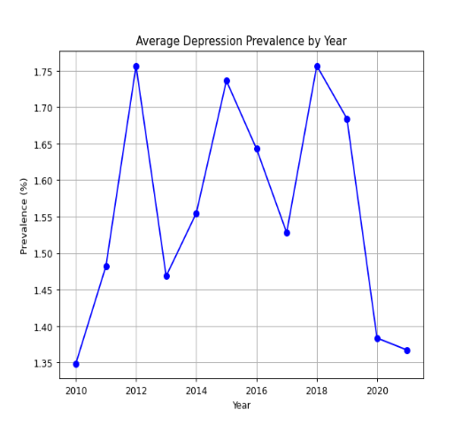
4.1 Line Plot: Depression Prevalence by Year

The first visualization is a line plot showing how depression prevalence has evolved over time. This plot is useful for identifying long-term trends in the data.

GitHub Gist

The line plot shows the average prevalence for each year in our dataset. Line graphs allow for easy trend identification, such as spotting whether the prevalence of depression is rising or falling and identify any sudden spikes or drops in the trend. For more complex data points or composite trends, having a trend line may be useful.

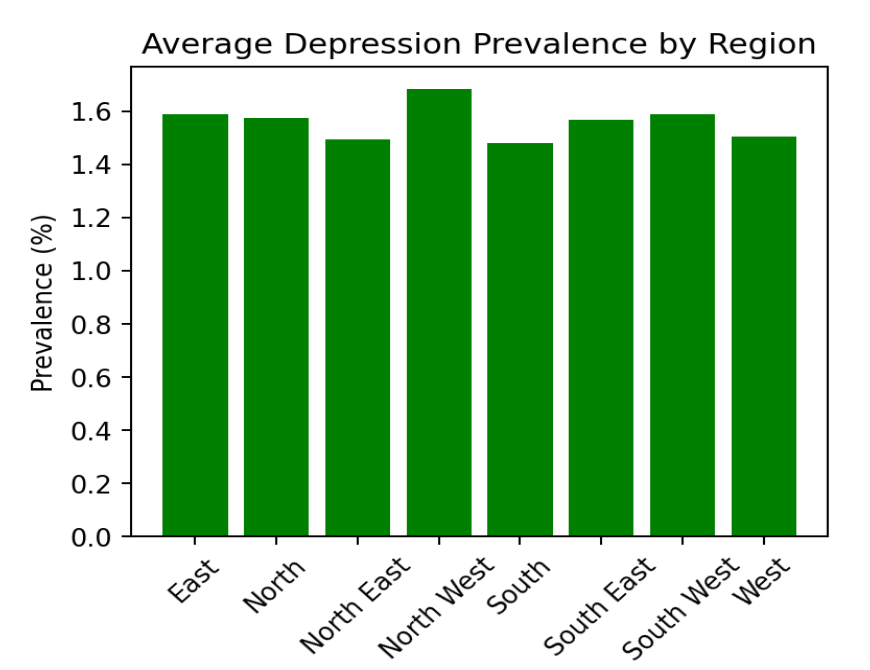
4.2 Bar Plot: Depression Prevalence by Region

Next, we create a bar plot to compare depression prevalence across different regions. Bar plots are particularly effective for comparing categorical data like regions.

GitHub Gist

The bar plot shows the average prevalence of depression for each region. This visualization allows you to quickly compare which regions have higher or lower rates of depression. It’s also useful for identifying regions that might need targeted public health interventions.

Conclusion:

This project provides a solid foundation for analyzing public health data using Python. Whether you’re studying epidemiology or working in the field, being able to calculate prevalence rates and present data visually is a crucial skill. You can now apply these techniques to other datasets and health-related challenges!

Humanities Moment

The featured image for this PyFriday Tutorial is Sleepy Kittens (1900) by Henriëtte Ronner-Knip (Dutch, 1821 – 1909). Henriëtte Ronner-Knip was a Dutch-Belgian Romantic artist renowned for her animal paintings, particularly of cats. Born into a family of artists, she became the primary financial supporter of her family, gained recognition for her work, and exhibited internationally, earning prestigious awards like the Order of Leopold and the Order of Orange-Nassau. Enjoy this tutorial? Please consider looking at our other offerings here at Broadly Epi!

Epi Explained: Understanding P-Values and Z-Scores

Epi Explained: Understanding Statistical Significance, P-Values, and Z-Scores

Statistical significance, p-values, and z-scores are fundamental concepts in statistics and research. They are crucial in fields such as medicine, psychology, and economics, helping researchers determine if their findings are due to chance or represent genuine relationships in the data. This Epi Explained aims to make these concepts more accessible by explaining them in detail and breaking down their importance in research.

Key Takeaways

What does a p-value of 0.05 mean?

A p-value of 0.05 means there’s a 5% chance that the results occurred due to random variation if the null hypothesis is true. If the p-value is lower than 0.05, the results are considered statistically significant.

What is the difference between a z-score and a p-value?

A z-score measures how far a data point is from the mean in terms of standard deviations, while a p-value quantifies the probability of obtaining the observed results if the null hypothesis is true.

Can a high p-value still be useful?

Yes. A high p-value suggests that the observed data could have occurred by chance, which means there might not be enough evidence to reject the null hypothesis. However, this can still provide valuable information, such as when a treatment shows no effect.

What Is Statistical Significance?

Statistical significance measures whether the results observed in a study are unlikely to have occurred by chance. It’s a key concept in hypothesis testing, which is a structured way to test ideas and assumptions in research. By determining statistical significance, researchers assess whether their findings support a particular hypothesis.

The Basics of Hypothesis Testing

Hypothesis testing involves two opposing statements:

Null Hypothesis (H₀): There is no effect or no difference between the groups being compared.
Alternative Hypothesis (H₁ or H_a): There is an effect or a difference between the groups.

The goal of hypothesis testing is to determine whether there is enough evidence to reject the null hypothesis in favor of the alternative hypothesis. Statistical significance helps to decide whether the observed data supports rejecting H₀.

How to Calculate Statistical Significance

To calculate statistical significance, researchers use a measure called the p-value. The p-value represents the probability of observing results as extreme as (or more extreme than) those obtained, assuming the null hypothesis is true. A low p-value indicates that the observed results are unlikely under the null hypothesis, signaling statistical significance.

Understanding the P-Value

The p-value, or probability value, is a key element in hypothesis testing. It helps quantify how likely the data would occur if the null hypothesis were true.

Interpreting P-Values

P-Value < 0.05: The results are considered statistically significant, meaning there’s less than a 5% probability that the observed data is due to random chance. Researchers may conclude that there is evidence in favor of the alternative hypothesis.
P-Value ≥ 0.05: The results are not statistically significant. This suggests that any differences or effects observed could likely be due to chance, and researchers usually cannot reject the null hypothesis.

It’s essential to remember that a p-value does not measure the probability that the null hypothesis is true or false. Instead, it shows the probability of the data assuming the null hypothesis is true. Additionally, while 0.05 is commonly used as the threshold, many researchers opt for stricter cutoffs, such as 0.01, depending on the context of the study.

Concerns About Overusing P-Values

In some fields, especially biomedical research, the reliance on p-values has been criticized. A significant p-value doesn’t always mean the effect is practically meaningful or important. This has led to calls for more nuanced approaches in interpreting statistical findings.

What Is a Z-Score?

The z-score, also known as the standard score, measures how far a particular data point is from the mean of the dataset, expressed in terms of standard deviations. It’s a crucial concept for comparing different values and calculating probabilities in statistics.

Z-Score Formula

The formula for calculating the z-score is:

$z = (X − μ) / σ$

Where:

X is the value being measured.
μ is the mean of the population.
σ is the standard deviation of the population.

Interpreting the Z-Score

Positive Z-Score: Indicates that the value is above the mean.
Negative Z-Score: Indicates that the value is below the mean.
The magnitude of the z-score (how large or small the number is) indicates how many standard deviations away the value is from the mean.

Real-World Application of Statistical Significance and Z-Scores

These concepts are widely used in research, particularly in clinical trials and other fields where decision-making relies on data. That said, even in day to day public health work, significance is frequency used to check the strength of association between health related outcomes and variables, determining if a cluster of healthcare encounters is to be seen as normal or a potential significant outbreak/issue, or to do program evaluation.

Example Problem: Drug Testing

Let’s say a study is testing whether a new drug lowers blood pressure. The null hypothesis states that the drug has no effect on blood pressure, while the alternative hypothesis suggests it does lower blood pressure.

After conducting the study with 100 patients, the researchers find that the drug reduces blood pressure by an average of 5 mmHg, with a p-value of 0.02. This indicates that there is only a 2% chance that this result could have occurred by chance if the drug had no effect, making the results statistically significant.

If the mean blood pressure change in the population is 0 mmHg, and the standard deviation is 10 mmHg, the z-score for the observed decrease can be calculated as:

$z = (5 − 0) / 10 = 0.5$

This means the observed blood pressure decrease is 0.5 standard deviations above the mean expected under the null hypothesis, providing additional support for rejecting the null hypothesis.

Conclusion

Statistical significance, p-values, and z-scores are essential tools for analyzing data and drawing valid conclusions in research. By understanding these concepts, you can assess whether observed effects are likely real or the result of random variation. Whether you’re involved in research or simply trying to understand scientific studies, grasping these ideas is key to making data-driven decisions.

Humanities Moment

The featured image for this Epi Explained is The Judgement Of Paris (1812) by Guillaume-Guillon Lethière (French, 1760 – 1832). Guillaume Guillon-Lethière, a French neoclassical painter born in Guadeloupe in 1760, was the son of a French colonial official and a “mulatto” mother. He studied under Gabriel François Doyen, competed in the Prix de Rome, and established a successful studio in Paris, rivaling Jacques-Louis David. Elected to the Académie and awarded the Légion d’honneur in 1818, he later became a professor at the École des Beaux-Arts, mentoring students who would often cultivate a reputation of their own.

As always, thank you for reading this installment of Epi Explained. If you’d like to learn more about Epidemiology, Public Health, or the skills needed to excel in it, please check out our other articles here.

Epi Explained: Understanding Prevalence

Epi Explained: Understanding Prevalence Rate

Measuring disease burden in a population is crucial to public health decision-making. One of the most fundamental metrics used is the prevalence rate. Understanding this concept is key for professionals and students alike, especially when studying the distribution and impact of diseases in communities.

Key Takeaways

1. How is prevalence different from incidence?

Prevalence measures the total number of existing cases in a population, while incidence focuses on new cases over a specific period.

2. What does a high prevalence rate indicate?

A high prevalence rate indicates that a disease or condition is widespread within a population. This may suggest a chronic health problem or an ongoing issue that requires targeted intervention.

3. Can a disease have high prevalence but low incidence?

Yes, diseases like diabetes or hypertension can have high prevalence but low incidence, meaning they are widespread but not many new cases are being diagnosed compared to the total number of existing cases.

What is Prevalence Rate?

The prevalence rate refers to the total number of individuals in a population who have a particular disease or condition at a specific point in time or over a defined period. It is a proportion that helps to illustrate the disease burden within a population, offering insights into how widespread a condition is.

Unlike incidence rate, which measures new cases, prevalence includes both new and existing cases. Therefore, it provides a snapshot of the overall disease burden.

Formula for Calculating Prevalence Rate

To calculate the prevalence rate, use the following formula:
Prevalence Rate (%) = (Number of existing cases / Total population) × 100
Where:

Number of existing cases refers to individuals who currently have the disease or condition.
Total population is the population group being studied (e.g., city, country, or age-specific group).

For example, if a town of 10,000 people has 500 individuals with a chronic disease, the prevalence rate would be:
Prevalence Rate (%) = (500 / 10,000) × 100 = 5%

Types of Prevalence

There are two main types of prevalence rates used in public health:

1. Point Prevalence

Point prevalence refers to the proportion of a population that has a disease at a specific point in time. It is often used in cross-sectional studies and helps public health officials assess the immediate burden of disease.

2. Period Prevalence

Period prevalence measures the proportion of a population that has a disease over a specific period, such as one year. This type of prevalence is useful when analyzing diseases that have fluctuating patterns, such as seasonal illnesses.

Why is Prevalence Rate Important?

The prevalence rate plays a vital role in understanding the public health impact of both chronic and acute diseases. Here’s why it matters:

Assessing healthcare needs: Prevalence rates help public health professionals allocate resources efficiently based on the disease burden in a community.
Tracking disease trends: Changes in prevalence rates over time can indicate shifts in disease patterns, treatment effectiveness, or the impact of public health interventions.
Comparing populations: Prevalence rates allow for comparison between different population groups, regions, or countries, providing insights into disparities in health conditions.

Factors Affecting Prevalence Rate

The prevalence rate can be influenced by several factors, including:

Incidence rate: A higher incidence (new cases) leads to an increase in prevalence unless offset by recovery or death.
Duration of the disease: Chronic conditions that last longer contribute to a higher prevalence rate compared to short-lived diseases.
Migration patterns: Movement of populations can affect the prevalence of certain conditions in a given area, especially if people with the disease migrate into or out of a region.

Prevalence Rate vs. Incidence Rate

It’s essential to distinguish between prevalence rate and incidence rate. While both are used to measure disease occurrence, they serve different purposes:

Prevalence Rate reflects the total number of cases (new and existing) in a population at a given time.
Incidence Rate measures the number of new cases occurring in a population during a specific period.

For example, if a disease like diabetes has a high prevalence rate, it indicates a significant ongoing burden, whereas a low incidence rate might suggest that fewer new cases are being diagnosed.

Real-World Applications of Prevalence Rate

Prevalence rates are used in various aspects of public health and epidemiology, such as:

Chronic disease management: Conditions like diabetes, hypertension, and asthma require ongoing management, and prevalence rates help to gauge the long-term burden of these diseases on health systems.
Infectious disease surveillance: Monitoring diseases like HIV, tuberculosis, or COVID-19 often involves tracking prevalence to understand how widespread the infection is in a given population.
Health policy formulation: Governments and health organizations use prevalence data to craft policies aimed at controlling or mitigating diseases, particularly when resource allocation is involved.

Conclusion

The prevalence rate is a crucial measure in epidemiology, offering insights into how common a disease is within a specific population. By understanding prevalence rates, public health officials can better allocate resources, assess treatment effectiveness, and plan disease prevention strategies. Whether you’re a student, researcher, or healthcare professional, mastering the concept of prevalence helps you interpret disease patterns and contribute to effective public health interventions.

Humanities Moment

The featured image for this installment of Epi Explained is Monks On The Appian Way (ca. 1865) by Elihu Vedder (American, 1836-1923). Elihu Vedder, an American artist known for his allegorical and symbolic works, spent much of his career in Europe, particularly Italy. His art, often dreamlike and mysterious, includes iconic murals and illustrations, notably for the Rubaiyat of Omar Khayyam, and he frequently returned to the U.S. for public commissions. Vedder eventually settled in Rome permanently a year after this work was completed.

Epi Explained: Understanding Incidence Rate

In epidemiology, the incidence rate is one of the most important measures for understanding the occurrence of new cases of a disease or condition over a specified period. While often associated with infectious disease, knowing how to calculate and interpret the incidence rate is crucial for making informed decisions about health policy and interventions for basically any realm that public health touches.

Top Takeaways

What is the difference between incidence rate and prevalence?
Incidence rate measures new cases of a disease during a specific time period, while prevalence measures all existing cases (both new and pre-existing) at a given point in time.
What is person-time?
Person-time is the sum of the time periods each individual in a study was at risk of developing the disease. It accounts for variations in how long each person is followed.
How do you interpret an incidence rate?
An incidence rate of 0.05 per year means that there are 5 new cases for every 100 person-years of follow-up.

What Is Incidence Rate?

The incidence rate refers to the frequency at which new cases of a disease occur in a specific population over a given time period. Unlike prevalence, which measures the total number of existing cases, incidence focuses solely on new occurrences, making it an essential tool for identifying and tracking emerging health threats.

Incidence Rate Formula

The formula for calculating the incidence rate is:

Incidence Rate = (Number of new cases / Population at risk) × Time

Where:

Number of new cases: The total number of new cases of the disease or condition occurring during the time period.
Population at risk: The group of individuals who are at risk of developing the disease during the study period (i.e., they do not already have the disease).
Time: The length of the observation period, often expressed in person-years to account for varying follow-up durations.

To understand incidence rate fully, it’s important to be familiar with a few related terms and concepts:

Person-Time

In many epidemiological studies, the population size can fluctuate, and the exact time each individual is at risk may vary. This is where person-time comes into play. Person-time is the sum of the periods during which each individual in the population was at risk. It accounts for differences in how long each person was observed, giving a more accurate representation of risk.

Cumulative Incidence vs. Incidence Rate

Although often used interchangeably, cumulative incidence and incidence rate are distinct concepts. Cumulative incidence measures the proportion of a population that develops a disease over a specified period, while incidence rate (also called incidence density, though rarely) accounts for the exact timing of new cases, using person-time in its calculation.

How to Calculate Incidence Rate: An Example

Let’s say we are investigating the incidence rate of a respiratory illness in a population of 10,000 individuals over a one-year period. During this time, 500 new cases were recorded. To calculate the incidence rate, we would use the following steps:

Identify the number of new cases: In this example, 500 new cases.
Determine the population at risk: The entire population is 10,000, assuming all individuals are at risk at the start of the year.
Specify the time period: The observation period is one year.
Apply the formula:
Incidence Rate = (500 / 10,000) × 1 year = 0.05 per year

In this case, the incidence rate is 0.05, or 5 new cases per 100 person-years.

Why Is Incidence Rate Important?

Incidence rates are essential in public health because they help health professionals:

Monitor disease trends: By comparing incidence rates over time or across different regions, we can detect potential outbreaks or changes in disease patterns.
Identify risk factors: Incidence rates allow researchers to assess whether certain populations are more vulnerable to a disease, helping target prevention strategies more effectively.
Evaluate interventions: By tracking incidence rates before and after an intervention, such as a vaccination campaign, we can measure the effectiveness of public health measures.

Limitations of Incidence Rate

While the incidence rate is a valuable tool in epidemiology, there are some limitations:

Population at risk accuracy: Determining the correct population at risk can be challenging, especially in dynamic populations where people may move in or out of the study area. Typically in the field, people will rely on Census or ACS estimates of age, sex, or other key demographics to estimate the population of interest. Likewise, combining this data with something like BRFSS which asks about specific behaviors, conditions and risk factors, may provide a slightly better estimate for an at risk population.
Chronic diseases: For chronic diseases that develop slowly, incidence rates may not provide the full picture since they focus only on new cases and not the burden of long-term illness. Due to similar reasons, certain conditions which may have a cultural taboo associated with it, or a newly discovered condition, may have suppressed or expanded incidence rates respectively. This is due to factors that are not due to the disease or the underlying cause of the disease itself.

Conclusion

The incidence rate is a cornerstone of epidemiology, providing insight into how often new cases of a disease occur within a specific population over time. By understanding how to calculate and interpret this rate, public health professionals can better identify emerging health threats, plan interventions, and allocate resources. Though there are limitations, particularly in tracking chronic diseases or some other conditions, the incidence rate remains a key metric for protecting and improving public health.

Humanities Moment

The featured image for this Epi Explained is Unsere Haustiere Pl.04 (1911) by Fritz Gareis jr. (Austrian, 1872 – 1925).
Fritz Gareis Jr. was an Austro-Hungarian artist and cartoonist known for his work on the satirical magazine “Götz von Berlichingen” and his comic strip “Bilderbogen des kleinen Lebens”, which featured the fictional Riebeisel family and is considered one of the first comics in continental Europe to use speech balloons. His comic became so popular that it continued after his death in 1925, drawn by Karl Theodor Zelger until 1934.

Thank you for reading this installment of EpiExplained on Incidence Rates. If you’d like to learn more about epidemiology, public health, or programming, please check out the rest of our available articles.

Epi Explained: What are Sensitivity and Specificity in Epidemiology?

Quick Takeaways

Sensitivity measures a test’s ability to correctly identify individuals with the disease.
Specificity measures how well a test correctly identifies individuals without the disease.
Sensitivity and specificity are key in reducing false positives and negatives, crucial for public health screening.
Predictive values (PPV and NPV) depend on the prevalence of the disease in the population.
Advances in diagnostic technology aim to improve the balance between sensitivity and specificity.

Sensitivity and specificity are two of the most critical metrics in epidemiology, essential for analyzing the accuracy of diagnostic tests and the effectiveness of public health screening programs. Whether you’re a public health professional, a student, or someone with a general interest in public health, understanding these concepts is vital for interpreting data and making informed decisions. This article delves into the core definitions of sensitivity and specificity, explains their real-world applications, and explores their importance in epidemiological analysis.

Understanding the Basics of Sensitivity and Specificity

Sensitivity: The Test’s Ability to Detect Disease

Sensitivity refers to a test’s ability to correctly identify individuals who have a specific disease. In epidemiological studies, a highly sensitive test ensures that most cases of the disease are correctly identified, reducing the likelihood of missed diagnoses. Sensitivity is mathematically expressed as:
$\text{Sensitivity} = \frac{ \text{True Positives} }{ \text{True Positives} + \text{False Negatives} }$
This equation calculates the proportion of individuals who test positive among those who truly have the disease. For example, a test with a sensitivity of 90% will correctly identify 90% of individuals with the disease, but it may miss 10%, leading to false negatives.

Example: Consider a tuberculosis (TB) screening program in high-prevalence regions. A sensitive test, such as the tuberculin skin test, is crucial to ensuring that cases of TB are detected early to prevent transmission. However, high sensitivity can sometimes lead to more false positives, especially in populations vaccinated with BCG.

Specificity: The Test’s Accuracy in Identifying Healthy Individuals

Specificity is the ability of a test to correctly identify individuals who do not have the disease. This metric is important in minimizing false positives. Specificity is calculated as:
$\text{Specificity} = \frac{ \text{True Negatives} }{ \text{True Negatives} + \text{False Positives} }$
A test with high specificity ensures that most healthy individuals are not incorrectly diagnosed with the disease. In epidemiological terms, specificity is important for confirming diagnoses and ensuring that healthy individuals are not misclassified as sick.

Example: In diagnosing HIV, tests with high specificity, such as confirmatory Western blot tests, are essential. These tests ensure that people who are not infected are not incorrectly diagnosed as HIV-positive, thus preventing unnecessary stress and treatment.

The Mathematical Foundations of Sensitivity and Specificity

Calculating Sensitivity

Sensitivity, as discussed earlier, is calculated by dividing the number of true positives by the sum of true positives and false negatives. This measure helps determine how effectively a test can identify individuals with the disease:
$\text{Sensitivity} = \frac{ \text{True Positives} }{ \text{True Positives} + \text{False Negatives} }$
For example, if a test detects 120 true positive cases of a disease but misses 30 cases (false negatives), the sensitivity of the test is:
$\text{Sensitivity} = \frac{ 120 }{ 120 + 30 } = 0.80$
This means the test has an 80% sensitivity, meaning it detects 80% of the true positive cases.

Calculating Specificity

Specificity is calculated by dividing the number of true negatives by the sum of true negatives and false positives. This calculation ensures we can evaluate how well the test identifies healthy individuals:
$\text{Specificity} = \frac{ \text{True Negatives} }{ \text{True Negatives} + \text{False Positives} }$
If a test correctly identifies 90 healthy individuals (true negatives) but misidentifies 10 healthy individuals as positive (false positives), the specificity would be:
$\text{Specificity} = \frac{ 90 }{ 90 + 10 } = 0.90$
This test has 90% specificity, meaning it correctly identifies 90% of healthy individuals.

Sensitivity and Specificity in Public Health Screening

The Role in Disease Control

In public health screening programs, sensitivity and specificity are crucial for disease control and prevention efforts. A sensitive test ensures that as many cases as possible are detected early, especially in high-prevalence conditions. Specificity, on the other hand, ensures that false positives are minimized, reducing unnecessary treatment and anxiety in healthy individuals.

Example: Consider diabetes screening. Tests like fasting glucose or HbA1c are used to detect the disease. A highly sensitive test ensures that most individuals with diabetes are caught early, but if specificity is too low, many individuals without diabetes may be incorrectly identified, leading to over-treatment and higher healthcare costs.

Balancing Sensitivity and Specificity for Optimal Screening

Balancing sensitivity and specificity is a significant challenge in public health screening programs. High sensitivity may lead to increased false positives, while high specificity may miss some true cases. For example, in cancer screening, such as mammography, balancing sensitivity (to catch as many cases as possible) and specificity (to reduce unnecessary biopsies) is critical to effective screening and healthcare system efficiency.

Sensitivity and Specificity in Predictive Values

Positive Predictive Value (PPV)

Positive predictive value (PPV) is the probability that a person with a positive test result truly has the disease. PPV is influenced by both the sensitivity and specificity of the test as well as the prevalence of the disease in the population. It is calculated as:
$\text{PPV} = \frac{ \text{True Positives} }{ \text{True Positives} + \text{False Positives} }$
Example: If a population has a low prevalence of disease, even a test with high specificity may produce a significant number of false positives, reducing the PPV.

Negative Predictive Value (NPV)

Negative predictive value (NPV) is the probability that a person with a negative test result truly does not have the disease. Similar to PPV, NPV is affected by the prevalence of the disease. It is calculated as:
$\text{NPV} = \frac{ \text{True Negatives} }{ \text{True Negatives} + \text{False Negatives} }$
For instance, in a population where the disease is rare, a test with high NPV is highly reliable in indicating that a negative result is truly negative.

Real-World Applications of Sensitivity and Specificity

Case Study: Sensitivity and Specificity in HIV Testing

HIV testing is an excellent example of how sensitivity and specificity are used to make crucial health decisions. Initial HIV screening tests, like enzyme immunoassays (EIAs), are designed to be highly sensitive, ensuring that nearly all HIV-positive cases are detected. Confirmatory tests, such as the Western blot, are then used to ensure high specificity, ruling out false positives.

Challenges in Achieving High Sensitivity and Specificity

While it is desirable to have tests with both high sensitivity and specificity, in reality, trade-offs are often made depending on the context. In some cases, public health programs may prioritize sensitivity to ensure that as many cases as possible are identified. In other situations, specificity may be prioritized to reduce unnecessary treatments and resource use. Lastly, there are occasions where the condition or disease itself when combined with volume and community can make it hard to establish a baseline for sensitivity or specificity.

Sensitivity and Specificity in Decision-Making

Sensitivity and Specificity in Clinical Decision-Making

Healthcare providers rely on sensitivity and specificity metrics to inform clinical decision-making. For example, in deciding whether to proceed with invasive diagnostic procedures, a highly specific test can help confirm the necessity of such measures, reducing patient risk and healthcare costs.

Public Health Policies and Sensitivity/Specificity

At the population level, public health policies often rely on balancing sensitivity and specificity to create effective screening guidelines. This balance ensures that healthcare resources are used efficiently while maximizing the health benefits of screening programs.

Common Misconceptions about Sensitivity and Specificity

Misinterpretation of Test Results

One common misconception is that high sensitivity or specificity alone ensures a perfect test. In reality, these metrics must be considered alongside other factors like disease prevalence and predictive values. For example, a test with high sensitivity but low specificity may result in many false positives, leading to unnecessary follow-up testing and treatment.

Confusing Sensitivity/Specificity with Predictive Values

It is essential to understand that sensitivity and specificity are not the same as positive predictive value (PPV) and negative predictive value (NPV). Sensitivity and specificity are intrinsic properties of the test itself, whereas PPV and NPV depend on the disease prevalence in the population being tested.

Improving Sensitivity and Specificity in Future Testing

Innovations in Test Design

Advances in diagnostic technology, such as machine learning algorithms and molecular diagnostics, are helping to improve both the sensitivity and specificity of tests. These technologies allow for more precise detection and classification of diseases, which is particularly valuable in the context of rare or complex diseases.

The Future of Public Health Diagnostics

As public health continues to advance, new diagnostic tools will enable better screening programs. These innovations will likely focus on optimizing sensitivity and specificity to ensure accurate diagnosis while minimizing false results. Such advancements are crucial for improving healthcare efficiency and patient outcomes globally.

Conclusion

Sensitivity and specificity are fundamental concepts in epidemiology, essential for understanding and interpreting diagnostic tests and public health screening programs. While both metrics are critical for determining test accuracy, they must be used in conjunction with other factors, such as disease prevalence and predictive values, to make informed public health decisions. As diagnostic technology continues to evolve, we can expect improvements in both sensitivity and specificity, leading to better health outcomes and more efficient use of healthcare resources.

For public health professionals and students, understanding these metrics is crucial for interpreting data and making sound decisions that affect population health. As testing continues to play a central role in disease prevention and control, sensitivity and specificity will remain at the heart of effective epidemiological analysis and decision-making.

Humanities Moment

The featured article for this image is Large Flowering Sensitive Plant. (1799–1807) by Robert John Thornton (English, 1768-1837). Robert John Thornton was an English physician and botanical writer, best known for his work “A New Illustration of the Sexual System of Carolus von Linnæus” (1797-1807), which included the celebrated “Temple of Flora.” Inspired by the work of Linnaeus and John Martyn’s lectures, he transitioned from studying theology to medicine, later practicing and lecturing in medical botany in London.

Thank you for reading this installment of EpiExplained. If you’re interested in learning more about Epidemiology, check out our other Epi Explained articles, or look at our other tutorials, research summaries, or software!

Epi Explained: Understanding Biases and Errors in Epidemiology

Quick Takeaways

What is the difference between bias and random error in epidemiology? Bias is a systematic deviation from the truth, while random error occurs by chance. Random error can be reduced by increasing the sample size, but bias requires methodological changes to correct.
How does selection bias affect a study? Selection bias arises when the participants in a study are not representative of the general population, potentially skewing the study’s findings.
What is a confounder in epidemiology? A confounder is a variable that affects both the exposure and the outcome, distorting the observed relationship between them.
What is the role of logistic regression in controlling confounding? Logistic regression is a statistical tool used to adjust for confounders by including them as variables in the regression model. This approach allows for the estimation of the association between the primary exposure and the outcome while controlling for the potential confounding effects of other variables. By incorporating both the exposure of interest and confounding variables as predictors in the model, logistic regression helps isolate the true effect of the exposure on the outcome.

Introduction to Biases and Errors in Epidemiology

In the field of epidemiology, ensuring the accuracy and reliability of research is vital for understanding health patterns and guiding public health decisions. Biases and errors—whether systematic or random—can distort study results, leading to inaccurate conclusions and possibly flawed public health policies. This article will explore key concepts related to biases and errors, including their mathematical underpinnings, and offer strategies for minimizing these issues in epidemiological research.

What is Bias in Epidemiology?

Bias in epidemiology refers to systematic errors that consistently skew the results of a study away from the true value. Unlike random errors, which occur by chance and can be reduced with larger sample sizes, biases are inherent to the study’s design or methodology.

Types of Bias

Systematic Error: A consistent error in measurement or methodology leading to a biased estimate of effect.
Random Error: Variability that occurs by chance and can be minimized through proper statistical techniques.

Mathematical Representation of Bias

Bias is often quantified using mathematical tools. For instance, the bias (B) of an estimator is the difference between the expected value of the estimator and the true value of the parameter being estimated:

$B(\hat{\theta}) = E[\hat{\theta}] – \theta$

Where:

$\hat{\theta}$ is the estimator,
$\theta$ is the true value,
$E[\hat{\theta}]$ represents the expected value of the estimator.

If the bias is zero, the estimator is considered unbiased.

Types of Bias in Epidemiology

Selection Bias

Selection bias arises when the participants selected for a study are not representative of the target population, which leads to skewed estimates. This often happens when certain groups are more likely to be included in the study than others.

Example: Case-Control Studies

In a case-control study, if certain cases are more likely to participate due to specific characteristics (e.g., accessibility to healthcare), the study may overestimate or underestimate the association between the exposure and the outcome.

Mathematical Illustration

The bias from selection can distort measures like the odds ratio (OR), calculated as:

$OR = \frac{(a/c)}{(b/d)} = \frac{a \times d}{b \times c}$

Where:

$a$ = number of exposed individuals with the outcome,
$b$ = number of exposed individuals without the outcome,
$c$ = number of unexposed individuals with the outcome,
$d$ = number of unexposed individuals without the outcome.

Information Bias

Information bias occurs when there is misclassification of exposure or outcome status due to errors in measurement. This can result from poor recall in interviews or inconsistencies in diagnostic testing.

Recall Bias

For instance, in recall bias, individuals with a disease may remember exposures more clearly than those without the disease, which can distort study findings.

Misclassification Error

Misclassification can be either differential or non-differential. Differential misclassification occurs when errors depend on the outcome or exposure status, often pushing the results in a particular direction. Non-differential misclassification usually biases results toward the null hypothesis.

Confounding

Confounding occurs when a third variable, the confounder, distorts the relationship between the exposure and the outcome. The confounder is associated with both the exposure and the outcome but is not part of the causal chain. This can lead to incorrect conclusions about the effect of the exposure on the outcome.

Example of Confounding: Air Pollution and Asthma

Imagine studying the relationship between air pollution (the exposure) and asthma (the outcome). Socioeconomic status (SES) could be a confounder if people of lower SES are more likely to live in polluted areas and also more likely to develop asthma for reasons unrelated to air pollution.

Mathematical Explanation of Confounding

To quantify confounding, epidemiologists calculate both a crude odds ratio and an adjusted odds ratio. The crude OR does not account for confounding, while the adjusted OR controls for confounding factors like SES.

Crude Odds Ratio

$OR = \frac{(a/c)}{(b/d)} = \frac{a \times d}{b \times c}$

Where:

$a$ = number of exposed individuals with the outcome,
$b$ = number of exposed individuals without the outcome,
$c$ = number of unexposed individuals with the outcome,
$d$ = number of unexposed individuals without the outcome.

Adjusted Odds Ratio Using Logistic Regression

To adjust for confounding, logistic regression models include the confounder in the equation:

$\log(OR) = \beta_0 + \beta_1 X + \beta_2 Z$

Where:

$\beta_0$ is the intercept,
$\beta_1$ represents the effect of the exposure $X$ ,
$\beta_2$ represents the effect of the confounder $Z$ .

Case Study of Bias and Error: Coffee Consumption and Heart Disease

Consider the relationship between coffee consumption and heart disease. Early studies suggested that coffee drinkers had higher rates of heart disease. However, when researchers adjusted for smoking—a known risk factor for heart disease—they found that the relationship between coffee consumption and heart disease was much weaker. Smoking acted as a confounder because it was associated with both coffee drinking and heart disease.

Effect of Confounding

The crude odds ratio (before adjusting for smoking) showed a strong association, but the adjusted odds ratio (after adjusting for smoking) demonstrated that the original association was largely due to confounding.

Crude Odds Ratio

$OR_{\text{crude}} = \frac{(a/c)}{(b/d)} = 3.5$

This suggests a 3.5 times higher risk of heart disease among coffee drinkers.

Adjusted Odds Ratio

After controlling for smoking:

$OR_{\text{adjusted}} = 1.2$

After accounting for smoking, the risk associated with coffee consumption was much smaller, indicating that smoking was a confounder.

Conclusion

Biases and errors can significantly impact the accuracy of epidemiological research. Systematic errors like bias distort results in predictable ways, while random errors occur by chance and can be reduced through appropriate statistical methods. Confounding presents an additional challenge, as it can create false associations between exposure and outcome. Understanding these issues, along with the mathematical methods to detect and adjust for them, is crucial for producing valid and reliable research in epidemiology.

Humanities Moment

This articles featured image is The Mishap by Jan Van Chelminski (Polish, 1851 – 1925). Jan Chełmiński, also known as Jan van Chelminski, was a Polish painter born Jan Władysław Chełmiński. He began his artistic studies at the Munich Academy of Fine Arts on April 14, 1875, and worked across Europe. In 1895, he moved to New York, after obtaining British citizenship in 1893. Chełmiński gained widespread recognition during his lifetime for his historical paintings, particularly those focused on military history and the Napoleonic Wars.

Want to learn more about concepts in Epidemiology? Check our backlog of Epi Explained articles, as well as research summaries and R/Python tutorials!

Epi Explained: What is the Difference Between Epidemic, Pandemic and Endemic?

In the realm of epidemiology, the terms epidemic, pandemic, and endemic are fundamental in describing the prevalence and geographic spread of diseases. These terms, often used in public health discussions, especially in the context of outbreaks like COVID-19, help professionals and the public understand the scale and scope of health threats. This Epi Explained delves into the definitions, distinctions, and examples of each, providing a comprehensive understanding for beginners.

Epidemic: A Localized Surge

Definition and Key Features

An epidemic refers to a sudden increase in the number of cases of a disease above what is normally expected in a specific area or population. The key characteristics of an epidemic include:

Localized Increase: Epidemics are often confined to a single community, city, or region.
Sudden Surge: There’s a rapid rise in disease incidence over a short period.
Temporal Pattern: Epidemics typically have a defined time frame, starting with a few cases that exponentially grow, peak, and eventually decline.

Examples

Some modern examples of epidemics are often those which are also vaccine preventable. For instance, in recent years some small Measles outbreaks have turned into state or multi-state epidemics in the United States. Measles, which was formally eliminated in the United States in 2000, still can be imported and cause sporadic outbreaks, from a couple of people to several hundred in some communities. It is important to also note that Epidemic does not necessarily equate to any level of severity or lethality; The term Epidemic can be from a disease causing 0 fatalities, or be highly fatal such as Smallpox or Ebola epidemics.

Pandemic: A Global Outbreak

Definition and Key Features

A pandemic is an epidemic that has spread over several countries or continents, usually affecting a large number of people. The defining aspects of a pandemic include:

Global Spread: Pandemics cross international boundaries, affecting people worldwide.
Massive Scale: The number of individuals impacted is significantly higher than in epidemics.
Duration: Pandemics often last longer than epidemics due to their wide geographical spread.

Examples

The COVID-19 outbreak, declared a pandemic by the World Health Organization (WHO) in March 2020, is the most recent example. It’s worth noting that even though there have been Epidemic COVID waves with some semblance of seasonality, there’s been consistent cases since 2020. The H1N1 (swine flu) in 2009 also reached pandemic status, as has some of the most famous disease outbreaks of all time like the so-called Spanish Flu of the 20th century.

Endemic: A Constant Presence

Definition and Key Features

Endemic diseases are constantly present in a particular geographic area or population. These diseases have predictable rates of incidence and prevalence over time. Characteristics of endemic diseases include:

Stable Incidence: The number of cases does not fluctuate significantly over time.
Geographic Specificity: Endemics are confined to specific areas due to environmental conditions, population immunity, and other factors.
Predictability: Health professionals can often predict the number of cases based on past data.

Examples

Malaria is endemic in parts of Africa due to the constant presence of the Anopheles mosquito. Similarly, chickenpox was considered endemic in many countries before the widespread use of the varicella vaccine.

Comparison and Contextual Application

Understanding the difference between these terms is crucial for response work. For instance, an epidemic requires immediate, localized interventions, while a pandemic might necessitate global collaboration and resource allocation. Recognizing a disease as endemic helps in developing long-term strategies, such as vaccination programs, to manage its spread. These should not be seen as fully separated categories however, as a proper intervention plan in public health emergency response divisions or for larger programs, should account for the most likely transition of categories for an outbreak and plan accordingly.

Transition from Pandemic to Endemic

A disease can transition from pandemic to endemic status as it becomes integrated into the regular pattern of diseases within a population. COVID-19 is an example where discussions about its potential shift to endemicity are ongoing, indicating the virus might circulate permanently until sufficient efforts and solutions are put forth for eradication. Historically in policy circles, this has been a point of argument against response measures including social distancing and other practical prevention activities, with the false equivalence of something no longer being a pandemic and it being any less dangerous to a population.

Conclusion

Epidemics, pandemics, and endemic diseases represent different scales and patterns of disease spread. While epidemics denote a sudden increase in disease cases in a specific area, pandemics indicate a global outbreak affecting a substantial portion of the world’s population. Endemic diseases, on the other hand, are a constant presence within a particular region. Understanding these differences enhances our grasp of public health strategies needed to combat infectious diseases, reflecting the importance of epidemiology in safeguarding global health.

Humanities Moment

The featured image for this Epi Explained was Study for the altarpiece of Saint Rosalie among the Plague-Stricken (ca.1657–60) by Carlo Maratti (Italian, 1625-1713). Carlo Maratta was an Italian painter whose work bridged the Late Baroque and Classical styles, primarily active in Rome where he became the preeminent artist following the death of Bernini in 1680. Maratta’s art was influenced by the classical ideals of Raphael and the Baroque dynamism of color, and he became well-known for both his religious and portrait paintings. He led the most prominent art studio in Rome, contributed significantly to the art community as the director of the Accademia di San Luca, and in his later years, turned to restoration work to cope with a decline in patronage.